While pre-training methods have gained popularity for sequence data in the natural language processing (NLP) space, equivalent experiments have been adopted in various different fields including Computational Biology. Here we cover some of these sequence models from Computational Biology in detail. As always, these summaries are from the original papers as well as some other fantastic resources linked below.
Section 1: Preliminaries - Sequences in Biology
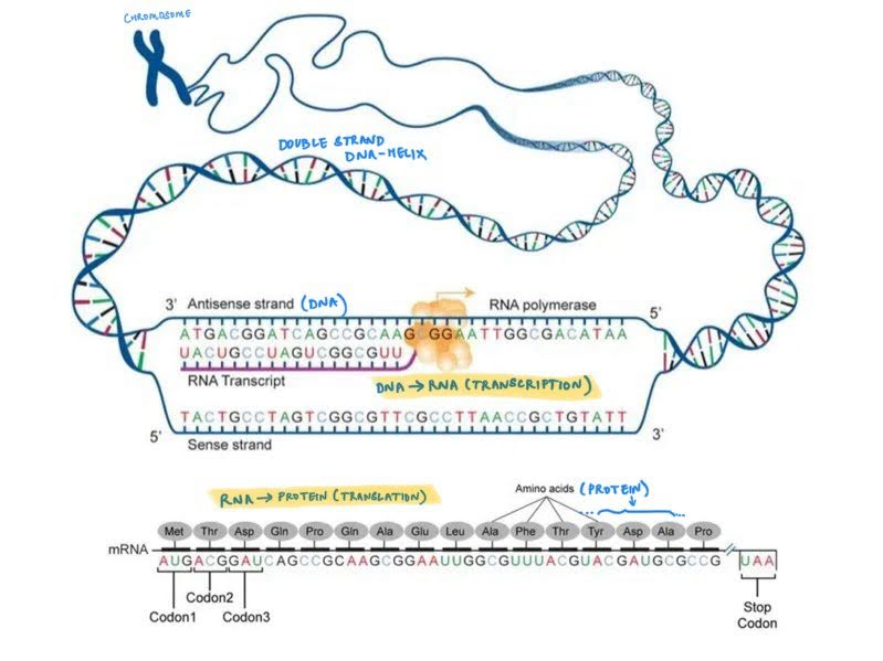
Nucleic acids structure The nucleic acids—DNA and RNA—are the principal informational molecules of the cell. DNA and RNA contain nucleotides, which consist of purines — adenine(A), guanine(G) — and pyrimidines — cytosine(C), thymine(T) for DNA or Uracil(U) for RNA — bases linked to phosphorylated sugars. These nucleotides undergo polymerization to form chains of nucleotides that are linked through phosphodiester bonds.
- Deoxyribonucleic acid (DNA) located in the nucleus is the primary genetic material for most living organisms. This contains two complementary strands of nucleotide chains that are linked together by hydrogen bonds where the base pairing is very specific: A always pairs with T and G with C. The complementary strands are called the template strands and the coding strands (Eg: Coding Strand: 5'-ATCGGTCAG-3', complementary non-coding (Template) Strand: 3'-TAGCCAGTC-5'). Since these strands are complementary, we study or process only the DNA’s coding strand. When viewed in 3D, the DNA always has a standard double helix structure, that is packed in various levels into the chromosome.
- Ribonucleic acid (RNA) participate in a number of cellular activities including, but not limited to protein synthesis. This single stranded chain of nucleotides is synthesised from DNA templates in a process called transcription. The RNA sequence is therefore identical to the coding strand of DNA except with Uracil (U) instead of Thyamine (T). The 3D structure of RNA depends on the its function.
Proteins Proteins direct virtually all activities of the cell — they serve as structural components of cells and tissues, transport of small molecules (like glucose and nutrients), transmitting information between cells, provide a defense against infections (antibodies) and act as enzymes. Proteins are polymer chains of amino acids, held together by the peptide bond. Each amino acid consists of a carbon atom (called the α carbon) bonded to a carboxyl group (COO–), an amino group (NH3+), a hydrogen atom, and a distinctive side chain that can be one of 20 different types. The amino acid sequence of a protein (consisting of 20 alphabets indicative of the 20 distinct amino acid side chains, also called ‘residues’) is only the first element of its structure, proteins adopt distinct three-dimensional conformations that are critical to their function. Proteins are synthesised using RNA templates (certain types of RNA called mRNAs) in a process called translation, where triplets of RNA nucleotide bases correspond to a single amino-acid with a distinct side chain.
The central dogma states that information flows from DNA → RNA → Protein. DNA serves as a template for synthesis of mRNA (transcription) and mRNA serves as a template for protein synthesis on ribosomes (translation).
A genome is the full set of genetic material in an organism encoded in the complete DNA sequence. For most multicellular organisms, every cell contains a complete copy of the genome. “Gene expression” is the process by which information from a gene (a segment of the DNA) is used to synthesize functional products, such as proteins or RNA molecules.
The nucleotide sequences (DNA/RNA) represent the genetic material through a sequence of 4 unique nucleotides A, G, C, T (U instead of T for RNA). A subset of a DNA sequence can map to an RNA sequence that can serve as a template for various functional components including proteins.
Protein sequences are represented as a combination of 20 unique amino acids that can adopt distinct 3D confirmations. The portion of the RNA that encodes proteins is mapped into amino-acids by grouping triplets of RNA nucleotides and matching them with the appropriate amino acid.
Section 2: Scale and complexities in Computational Biology sequences
DNA and RNA chains contain only 4 unique nucleotide bases, and the chains in proteins contain only 20 unique amino acids. There also seems to be direct mapping from DNA → RNA → Proteins, so learning representations for these sequences should be straightforward right? Not quite. [1][2][3]
- Unknown concepts of vocabulary: Current day NLP contains characters that are grouped into identifyable “words” that contain meanings, all of which are stored in a vocabulary. While the DNA/RNA sequences contain only 4 unique bases (and proteins contain only 20 unique AAs), their grouping into functional units (of variable lengths or patterns) is invisible to us and needs to be learnt; we are working with a hidden vocabulary. Some sections of the genome are known to map into proteins based on triplets of bases that correspond to amino acids. Other sections of DNA have known regulatory functions (promoters, ehancers, etc) based on common patterns studied across organisms. However, not all sections of the genome have a consistent/known mapping to structure or regulation. The learnt sequence representations need to learn these implicit meanings.
- The same genome can be processed differently: In alternative splicing, the same DNA sequence can be split in multiple different ways. Depending on the starting position and the different introns (regions retained for protein translation) and exons (non-coding regions of DNA that are disregarded for protein translation) within the same gene, we could arrive at three completely different proteins with different structures from the same DNA sequence. Additionally, despite the same underlying genome in all cells of the body, cell types, structure and functions exhibit extraordinary diversity. This diversity is made possible by the fact that cells use different subsets of the genome, regulated by epigenomics. The learnt sequence representations need to capture these diverse variations.
- Very long context windows: Regulatory sequences for a gene, can be located very far away from the gene on the genome, sometimes thousands of kilobases away. This is possible because of DNA looping which allows a transcription factor bound to a distant enhancer to interact with proteins associated with general transcription factors at the promoter. Similarly, protein sequences also contain long-range dependencies due to folding. We may want to capture these relationships between a gene and its enhancer (or two distant amino acids in a protein) but that’s only possible with very long context windows in our architecture.
- Single nucleotide polymorphisms A SNP is a variation in a DNA sequence where a single nucleotide is different from the normal sequence. While this seems to be inconsequential, they can have adverse consequences for diseases and drug responses of the body. So while our representations need to succintly capture structure/function, they ideally also need to still encode these nuanced changes at a single nucleotide level.
Section 3: Nucleotide representation learning: “Sequence modeling and design from molecular to genome scale with Evo”
Evo is a 7b parameter single-nucleotide resolution genomic foundational model (a DNA ‘languge’ model) with a context length of 131 kilobases, trained using 2.7 million prokaryotic and phage genomes. It is trained auto-regressively, to predict the next token given a nucleotide sequence. [2]
By virtue of being trained using nucleotide sequences, it is naturally multimodal (DNA or RNA generations can be translated to proteins) and inherently multi-scale (prediction/generation at molecular scale, systems scale or genome scale).


Section 3.1: Evo Pre-requisites
Section 3.1.1: Evo Prerequisites 1: CRISPR-Cas system and gene editing
CRISPR-Cas is an adaptive immune system in bacteria and archaea. It is composed of CRISPR (Clustered Regularly Interspaced Short Palindromic Repeats) repeat spacer arrays and CRISPR-Associated (Cas) genes that encode Cas proteins. When a virus infects a bacterium, the bacterium can store a snippet of the viral DNA (called a spacer) in its genome within the CRISPR array. This serves as genetic memory of past infections. When attacked by the same virus again, the corresponding spacer is used to generate a guide RNA that binds to a specific sequence in the viral DNA, and directs a Cas nuclease (nuclease cleaves a nucleotide chain) protein here to make cuts at this location. This system has been re-purposed across the bioinformatics field as a gene editing mechanism.
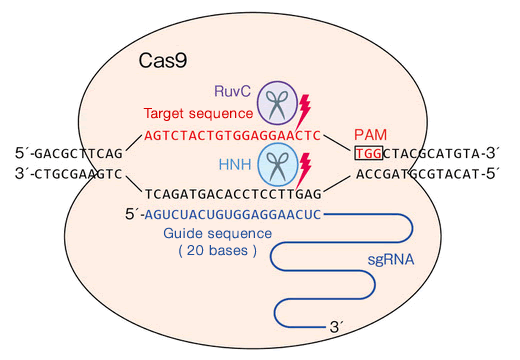
- Types of CRISPR-Cas: The current known CRISPR-Cas taxonomy consists of 5+ types and 15+ subtypes based on the target sequences and the types of cuts made by these systems. Of these, the CRISPR-Cas9 system (Type II) that uses the cas9 protein as the nuclease, is the most commonly used for gene editing, and targets double-stranded DNA, making blunt double stranded cuts.
- Structure of the system: The system typically contains cluster of Cas genes (genes that encode the Cas proteins), non-coding RNAs, and an array of repetitive elements. Between these repetitive elements are short variable-length sequences called protospacers. The repeats and spacers together form the CRIPSPR RNA array that contains the “guide” RNAs, transcription from this array forms the crRNA molecules, bound by the Cas protein to form a complex. [4][5]
- In the target DNA that is to be cleaved, the protospacer requires a protospacer-adjacent-motif (PAM) sequence for the Cas protein to bind and make cuts. The PAM sequence helps the Cas protein differentiate between foreign DNA (like viral DNA) and the host's own DNA. The CRISPR-Cas system only targets DNA sequences that are followed by the appropriate PAM, that varies for each type of system based on the PAM interacting domain present in the Cas protein. For Cas9 for example, the PAM sequence required in the target DNA is the NGG sequence (where N is any nucleotide). [4]
- The CRISPR-Cas9 system also contains an additional required auxiliary trans-activating crRNA (tracrRNA) that facilitates the processing of the crRNA array into discrete units.
The CRISPR-Cas loci is a region of the genome that contains both CRISPR array and the gene encoding the Cas protein.
CRISPR-Cas9 system (Figure source link)

- Using CRISPR-Cas9 for experimental gene editing:
- The crRNA and tracrRNA can be fused together to create a chimeric, single-guide RNA (sgRNA). Cas9 can thus be re-directed toward almost any target of interest in immediate vicinity of the PAM sequence by altering the 20-nucleotide guide sequence within the sgRNA. This sgRNA is constructed and functionally validated as per the gene-editing requirement. Typically, the sgRNA and the mRNA encoding the cas9 protein is injected into the target environment for gene editing.
- The double stranded breaks (DSBs) introduced by the Cas9 proteins are then repaired (or “edited”) using DNA repair pathways like NHEJ, or the HDR pathway that can use a user-controllable repair template.
- Creating new CRISPR-Cas systems: While there are a number of CRISPR-Cas systems that have already been discovered, people are always on the lookout to discover/engineer new CRISPR-Cas systems that have improved delivery (Eg: by reducing the size of the delivering Cas molecules) or improved target specificity (reducing the off-target cleavage). [6]
Section 3.1.2: Evo Prerequisites 2: MGE and Insertion sequences IS200/IS650
Mobile Genetic Elements are a category of DNA sequences that can jump within or between genomes. Amongst these, Transposable elements (TEs), also known as "jumping genes," are DNA sequences that move from one location to another within the genome. Class 2 TEs are characterized by the presence of terminal inverted repeats about 9 to 40 base pairs long, on both of their ends - one of the roles of these repeats is to be recognized by the enzyme transposase. “Insertion sequences” are a type of class II TE’s that are compact and encode only the elements required for their transposition
The IS200/IS650 Insertion sequences: These category of IS’s contain terminal imperfect palindromic structures instead of inverted repeats at both their ends. Unlike classical IS family members that transpose via the ‘cut and paste’ mechanism, this family transposes via a ‘peel and paste’ mechanism using single-stranded DNA (ssDNA) intermediates (instead of double stranded intermediates).
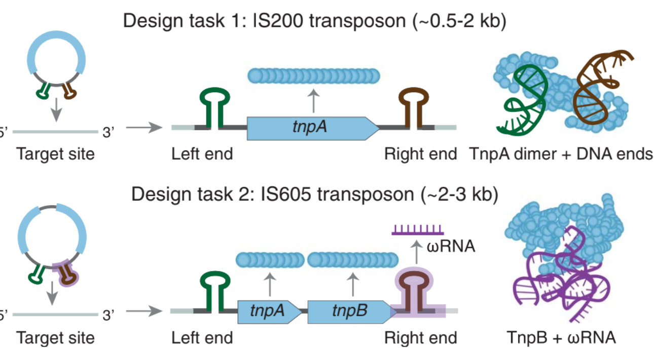
- IS200: Encodes the tnpA transposase that facilitates the peel-and-paste mechanism: it recognizes the terminal palindromic sequences and mediates the cleaving and rejoining of ssDNA.
- IS605: Encodes (a) The tnpA transposase (b) An additional open reading frame (ORF) that encodes tnpB, which is an RNA-guided endonuclease and (c) The ωRNA that guides tnpB to its DNA target.
Section 3.2: Evo - architectural and training details
One of the primary challenges of training at a single nucleotide resolution, with the appropriate context window (thousands of kilobases, see section 2 above) is the computational cost of the transformer architecture which scales quadratically with the sequence lengths.
Section 3.2.1: The Hyena Operator and Hyena layers

The Evo model uses the striped hyena architecture. This is a hybrid model that contains hyena operator layers, mixed in with a few attention layers that use RoPE to include positional information. The hyena operator is a replacement for attention, that combines long convolutions and element-wise gating over long context windows (at a sub-quadratic complexity) while still maintaining the desireable property of being input dependent. The hyena operator is useful for when you need very long context windows, and is more efficient that regular attention layers. To begin with, the input is projected into 3 streams (similar to attention) using dense layers on the channel dimension, and short-convolutions on the sequence dimension. Two of these streams are gated (multiplied) together, and a long convolution is applied, after which this is gated to the third stream. [2][7]
The long convolution (with a context window the size of the input) is implemented by
(a) Splitting the full size kernel into a weighted sum of continuous basis functions (of timestep). That is, which spans a subspace of possible values for the full kernel. Learning these weights is equivalent to its own mini neural network, and is much smaller than learning the full long convolution kernel
(b) The convolution is applied in the frequency domain with FFT (as element-wise multiplication) to make it more time efficient, and transformed back to the time domain. [2][7]
Section 3.2.2 Scaling laws - compute optimal analysis

Compute-optimal analysis studies the best performance of a pretraining run given a compute budget (typically indicated in floating point operations FLOPs) - the compute budget needs to be optimally split between the model size and the dataset size. For fixed compute budgets, the model size and the number of tokens is varied to study the perplexity metric; then a second order polynomial curve is fit to the datapoints, to identify the optimal allocation of model size and training tokens at the given compute budget. These scaling laws were studied for the StripedHyena architecture and also the Transformer++ architecture, the Mamba architecture and the Hyena architecture (Note: this study is done specific to using nucleotide sequences as input). [2]
Perplexity is a measure of a language model’s uncertainty of a sequence and is defined as the exponential of the negative log-likelihood of the sequence. Note that perplexity is defined for auto-regressive/causal-language models as
If a model’s max input size is
k, we then approximate the likelihood of a token by conditioning only on the k−1 tokens that precede it rather than the entire context.
The state-space and the hyena architectures had much better scaling (lowest eval perplexity) that the transformer architectures, and the authors observed stable training for StripedHyena throughout all the studied model sizes and learning rates. The authors estimated 250 billion to be the compute-optimal number of tokens for Evo 7B given the floating point operation (FLOP) budget. [2]
Section 3.2.2 Training the Evo Model
- Evo comprises 32 blocks at a model width of 4096 dimensions. Each block contains a sequence mixing layer, and a channel mixing layer. In the sequence mixing layers, Evo uses 29 hyena layers, interleaved with 3 rotary attention layers. For the channel mixing layers, Evo uses gated linear units, and normalizes inputs to each layer using RMS normalization.
- During pretraining, the model uses a vocabulary size of 4 tokens, the nucleotide sequence is tokenized and passed through an embedding layer, before being fed to the striped hyena architecture model. Evo predicts the likelihood of the next token given a sequence of tokens, referred to as autoregressive modeling
- The model is trained using data from the OpenGenome dataset that contains (i) bacterial and archaeal genomes from the Genome Taxonomy Database (GTDB) (ii) curated prokaryotic viruses from the IMG/VR v4 database (iii) plasmid sequences from the IMG/PR database. (Note: Evo does not use eukaryotic sequences).
- Evo is pre-trained in 2 stages: first with a vocabulary size of 8k, then with a size of 131k; this reduces the overall train time. Overall, Evo was trained using 340B tokens, equivalent to 1.13 epochs. Evo uses sequence packing to sample the data for training so that multiple smaller sequences can be joined with the EOS token if they are smaller than the context window.
Section 3.3: Evo - Results (Zero-shot and downstream training)
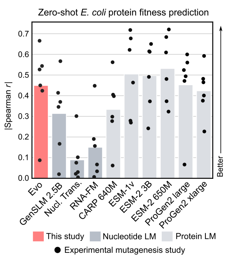
- Protein function prediction (zero-shot): The authors compile proteins and and corresponding fitness-values from relevant DMS studies, which introduce an exhaustive set of mutations to a protein coding sequence and then experimentally measure the effects of these mutations on various fitness values (fitness value is one quantify functional activity).
- Typically for protein models, the language model likelihood of the amino-acid sequence is used to predict the experimental fitness score. Note that Evo was not trained on amino-acid sequences but nucleotide sequences. Where there are multiple nucleotide sequences for a single protein sequence due to different codon usage, the nucleotide language models were evaluated on each unique nucleotide sequence and the protein language models were evaluated on the coding sequence corresponding to each unique nucleotide sequence.
- Authors compare Evo to two genomic DNA language models: GenSLM 2.5B and the Nucleotide Transformer, and several protein language models: CARP, ESM-1, ESM-2, ProGen2.
- For zero-shot function prediction, the authors consider the Spearman correlation co-efficient between the language model (LM) likelihood and the experimental fitness value — this measures how well the relationship between the variables can be described using a monotonic function. The t-statistic is a number that tells you how far your observed result is from the result expected in the null hypothesis, and the P-value is the probability of getting a result at least as extreme as the one you observed, if the null hypothesis were to be true.
- On DMS datasets of prokaryotic proteins, Evo’s zero-shot performance exceeded all other nucleotide models. Evo also reaches competitive performance with leading protein-specific language models.
Figure: Spearman correlation coefficient between fitness and perplexity, bar height
indicates the mean; each dot indicates a different DMS study

- Using ncRNA DMS datasets, authors show that Evo is also able to perform zero-shot fitness prediction for mutational effects on ncRNAs (like ribosomal RNAs and tRNAs), outperforming all other nucleotide language models at this task.
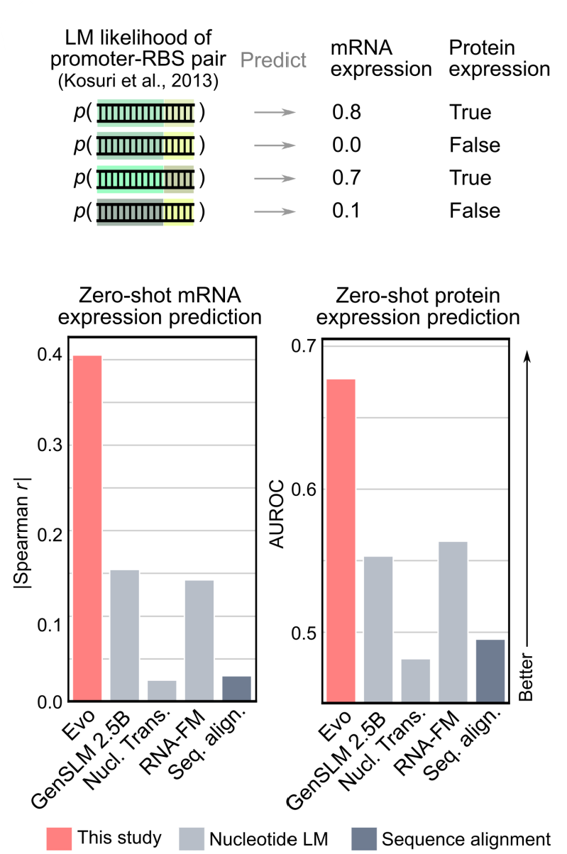
- Regulatory DNA Gene Expression Prediction “Gene expression” is the process by which information from a gene (a segment of the DNA) is used to synthesize functional products, such as proteins or RNA molecules. Gene expression is measured by quantifying the amount of mRNA or protein in a cell. One way to study gene expression is to study the transcriptome: i.e., at a given time how many copies of a given mRNA (corresponding to a gene) are present in the cell.
- For this task, the authors use a dataset of 5k+ promoter sequences with associated expression activity-labels for training data, and several thousand promoter sequences from 3 different studies for test data. (A promoter is a DNA sequence upstream of a gene that initiates transcription, that is by RNA polymerase and associated sigma factors, it controls transcription). Additionally, the authors also obtain a test set of promoter-RBS sequences (An RBS - Ribosome Binding Site - is a sequence on the mRNA, just upstream of the start codon ‘AUG’, that aligns the ribosome with the start codon, it controls translation); this study contains protein expression information in addition to mRNA expression.
- The authors evaluated both the zero shot predictive performance (based on sequence likelihood), and trained a supervised activity prediction model with (a) one-hot encodings of promoter sequences (b) Evo embeddings - the output of the last hidden layers. The authors train both a ridge regression model and a 2-layer convolutional neural network.
- Evo’s zero-shot likelihoods had non-negligible correlation with promoter activity across the four test studies (Spearman=0.43), exceeding that of the GC content and the zero-shot likelihoof of the GenSLM model. Across both the supervised model architectures, the Evo embeddings substantially outperform the one-hot embeddings, indicating Evo pretraining builds representations that are useful for function prediction.
- For the protein expression task, evo’s zero- shot likelihoods of the RBS sequence alone had weak correlation with protein expression (Spearman r = 0.17). However, when concatenating the promoter and RBS sequence together, Evo’s zero-shot likelihoods improved substantially (Spearman r = 0.61); beating GC content, zero- shot GenSLM likelihoods, and RBS calculator, a SOTA protein expression predictor.

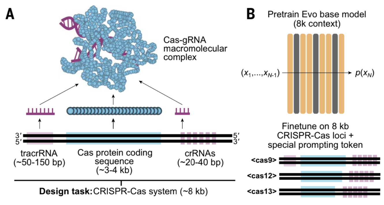
- Generating CRISPR-Cas systems (fine-tune): To evaluate whether evo can generate functional complexes that involve interactions between distinct molecular modalities, the authors fine-tuned Evo on a dataset of ~73k genomic loci containing CRISPR-Cas sequences (see Section 3.1.1 above). During fine-tuning, the authors add special prefix prompt tokens for the Cas9, Cas12 and Cas13 type loci to guide generation at test time.
- After training, the authors performed standard temperature-based and top-k autoregressive sampling to generate CRISPR-Cas systems, for downstream extraction and analysis. Sampling 8kb sequences using each of the three Cas token prompts resulted in coherent generations containing Cas coding sequences and CRISPR arrays corresponding to the expected subtype. For the generated CRISPR-Cas systems, the prodigal tool is used to identify Open Reading Frames (ORFs, regions that possibly code proteins). pHMMs trained on known Cas subtypes are used to detect if these ORFs resemble known Cas proteins. The MinCED package is then used to identify CRISPR arrays in the sampled sequences. The generated sequences with both Cas ORFs and CRISPR arrays were then aligned against the training data to identify closest matches amongst the training sequences.
- For experimental validation, generated Cas9 systems with <90% sequence identity to the closest training datapoint was retained. These sequences are then scored according to even distribution of mismatches with the closest aligned training samples. The top 2000 sequences are then folded with Alphafold2, and then filtered based on the pLDDT score, presence of a tracrRNA, and the presence of RuvC and HNH domains in the Cas9 ORF. 11 selected sequences are evaluated using an initial in vitro transcription translation assay followed by the introduction of a DNA target containing an NGG protospacer adjacent motif (PAM) sequence.
- Out of these, one of the generations called Evo-Cas9-1 showed robust activity, and recombinant expression of EvoCas9-1 paired with chemically synthesized Evo-generated sg-RNA showed comparable in-vitro cleavage activity to the canonical SpCas9 paired with SpCas9 sgRNA. EvoCas9-1 amino acid sequence shares 79.9% identity with the closest Cas9 in the database of Cas proteins used for model fine-tuning and 73.1% identity with SpCas9. Evo-designed sgRNA is 91.1% identical to the canonical SpCas9 sgRNA and exhibits secondary structure differ- ences in the two terminal stem loops.
Figure: (A) Protein coding genes and ncRNA found in the EvoCas9-1 CRISPR system, determined by pHMMs abd CRISPR array prediction algorithms (B) Predicted secondary structure of the sgRNA from Evo-Cas9-1 - letters in red show the deviation from the SpCas9 sgRNA (C) AF3 predictions of EvoCas9-1 aligned with Sp-Cas9-1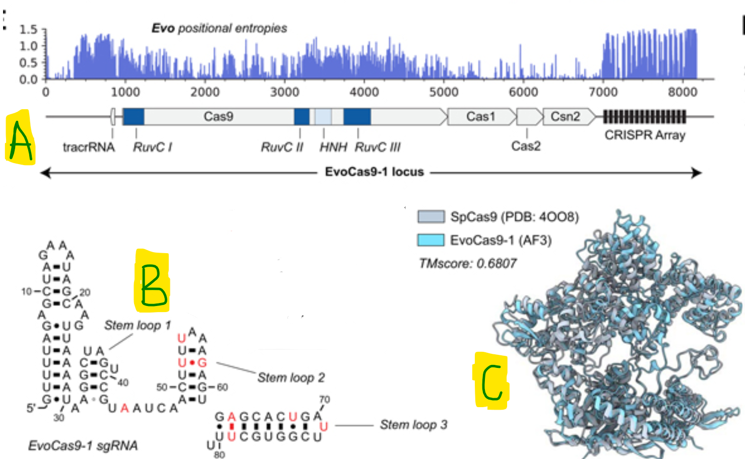
- After training, the authors performed standard temperature-based and top-k autoregressive sampling to generate CRISPR-Cas systems, for downstream extraction and analysis. Sampling 8kb sequences using each of the three Cas token prompts resulted in coherent generations containing Cas coding sequences and CRISPR arrays corresponding to the expected subtype. For the generated CRISPR-Cas systems, the prodigal tool is used to identify Open Reading Frames (ORFs, regions that possibly code proteins). pHMMs trained on known Cas subtypes are used to detect if these ORFs resemble known Cas proteins. The MinCED package is then used to identify CRISPR arrays in the sampled sequences. The generated sequences with both Cas ORFs and CRISPR arrays were then aligned against the training data to identify closest matches amongst the training sequences.


- Generative design of transposon systems (fine-tune): The authors fine-tune Evo on 10K+ IS605 elements and 200K+ IS200 elements in their natural sequence contexts.
- Using the fine-tuned model, the authors compute the entropy of conditional probabilities for naturally occuring IS200/IS605 in each position in the loci. Although the model was trained without any explicit labeling of MGE boundaries, the authors observe a sharp increase in entropy in the 3’ end of the boundary. A high entropy region means the model is uncertain, often reflecting boundaries, non-coding regions, or variable tails; here this signifies that the model is actually learning boundaries of these systems.
- Categorical jacobian analysis: The authors compute a “categorical jacobian” for naturally occuring IS200/IS605 using the logits from the fine-tuned Evo model as follows:
- Using the model, the authors compute the logits at each position for an input sequence (normally done for auto-regressive models using causal attention masking). Note that this tensor is of size . Next, the same tensor is computed for a mutation at each point (in the sequence L) into any of the other 4 nucleotide bases, and a difference between the original logits and logit values for these mutations are stored in a tensor. This tensor is centered and symmetrized. This tensor is turned into a ‘couplings map’ with a euclidian magnitude at each position in the sequence dimensions, the values for all nucleotide mutations are square-summed. Each entry in this matrix is seen as representing position coupling, a larger value indicates greater coupling between positions.
- The authors observe that the model uses information from one end to specify the other, meaning the model has understood the linkage between the terminal elements in these isotransposon systems.
- The fine-tuned model is used to generate IS200/IS605 systems using standard temperature based top-k autoregressive sampling. The generated sequences were analysed for coding sequences and ORFs,and for the presence of TnpA, TnpB and ωRNA using standard bioinformatics tools. These sequences are then aligned back to the training set and a representative subset binned by distance from the training set is selected. The respective IS200-like and IS605 like sequences are then folded using ESM fold. To select sequences for experimental validation, the subset of sequences are further filtered based on similarity to natural systems.
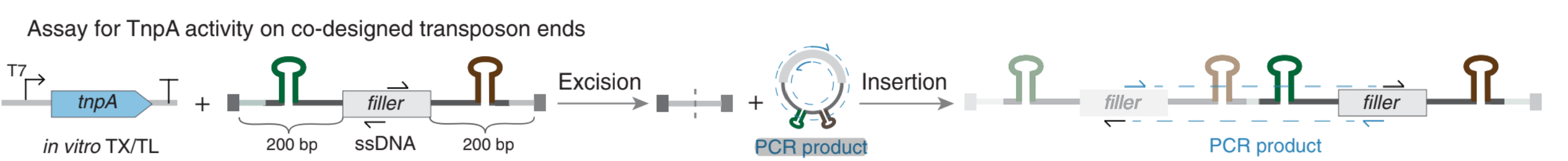
- A small subset of these systems are selected for experimental validation. This is done using assays to determine whether these designs showcase TnpA-mediated excision and insertion. The TnpA protein produced through in-vitro transcription and translation from these systems are incubated with an ssDNA substrate containing the left and right ends of these systems. PCR primers are designed to amplify DNA where excision has occured, and insertion has occured to test the fucntionality of these generated systems. 11 out of the 24 Evo-generated IS200-like elements and 3 out of 24 Evo-generated IS605-like elements demonstrated evidence of both excsision and insertion.


Section 4: Protein Representation Learning with the ESM family and ESM3
Studies like ProtTrans were one of the first few to explore the use of protein LMs (language models like T5, BERT, TransformerXL, etc) to extract features from individual protein sequences rather than using Multiple-Sequence-Alignments (MSA). These models trained in a self-supervised pretraining fashion (on UniRef50, UniRef100 and BFD) were then used as feature extractors for downstream tasks like per-residue protein secondary structure prediction, protein-level property prediction, etc. The similarly trained transformer-based ESM-1 model contained a detailed study of learnt representations (across use-cases like homology, alignment and biohemical properties), and similar performance on secondary structure prediction and protein contact prediction. [8]
Section 4.1: ESM3 pre-requisites — ESM2 and ESMFold
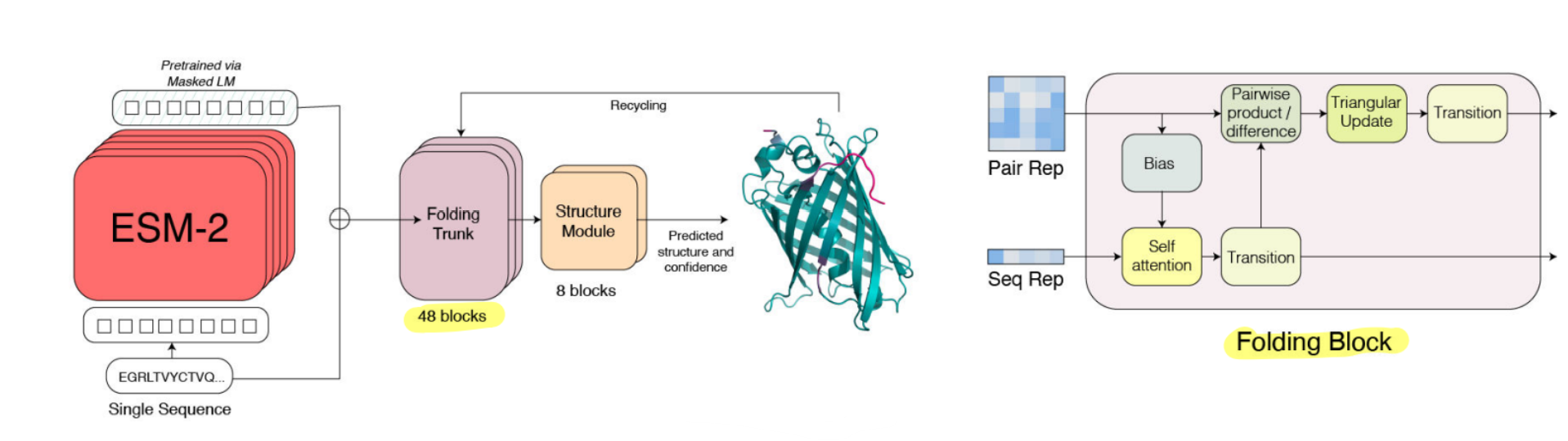
ESM2 had the ESM family of models scaled up to the largest known protein language models at the time; and additionally introduced ESMFold. ESMFold consisted of the ESM model representation combined with a modified Alphafold2 strcuture prediction module, to enable 3D protein structure prediction from single-sequence representations, that had comparable performance with state of the art MSA-based models like Alphafold2 while being an order of magnitude faster. [9]
- The ESM-2 model: The ESM-2 model with just150M parameters performed much better than ESM-1b (650 Million parameters). The newer ESM-2 architecture, while still a BERT-based transformer architecture used RoPE based learnt positional encodings instead of the static sinusoidal encodings of ESM-1b, and used an updated UniRef50 dataset. Additionally, the authors scaled ESM-2 from 8M parameters all the way to 15 B parameters, and show a consistent decrease in the language model perplexity, as they scale up. 🪢
Unlike the perplexity of auto-regressive models described above, masked models have a perplexity approximate. The non-deterministic approximate requires a single-pass to compute the exponential log-likelihood of the tokens in the mask. Since the “mask” is a random set, the same sentence could give different perplexity values. For the deterministic version, the “pseudo-perplexity” computes the log-likelihood of the sentence by masking one word at a time (requiring multiple forward passes with different masks), averaging, and taking an exponential of this value.
- The ESMFold model: To incorporate the ESM model protein sequence representations into the Alphafold2 structure prediction framework (a) The authors replace the Evoformer block with a single-sequence based block called the “folding block” — the axial attention in the evoformer required to process MSAs is replaced with the standard attention (b) The authors remove the use of templates from Alphafold2.

- ESM2 and ESMFold results
- The 15B parameter ESM-2 model has lowest validation perplexity and highest TM-score on CASP14. The 150M parameter ESM-2 models (and all larger models) outperform the 650M ESM-1b model. The 650M parameter ESM-2 model is comparable with the 3B parameter Prot-T5-XL-UniRef50 model, suggesting
ESM-2 models are far more parameter efficient.
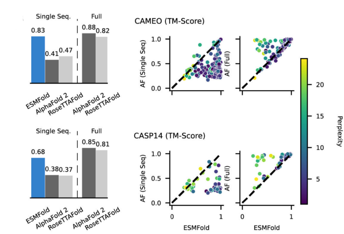
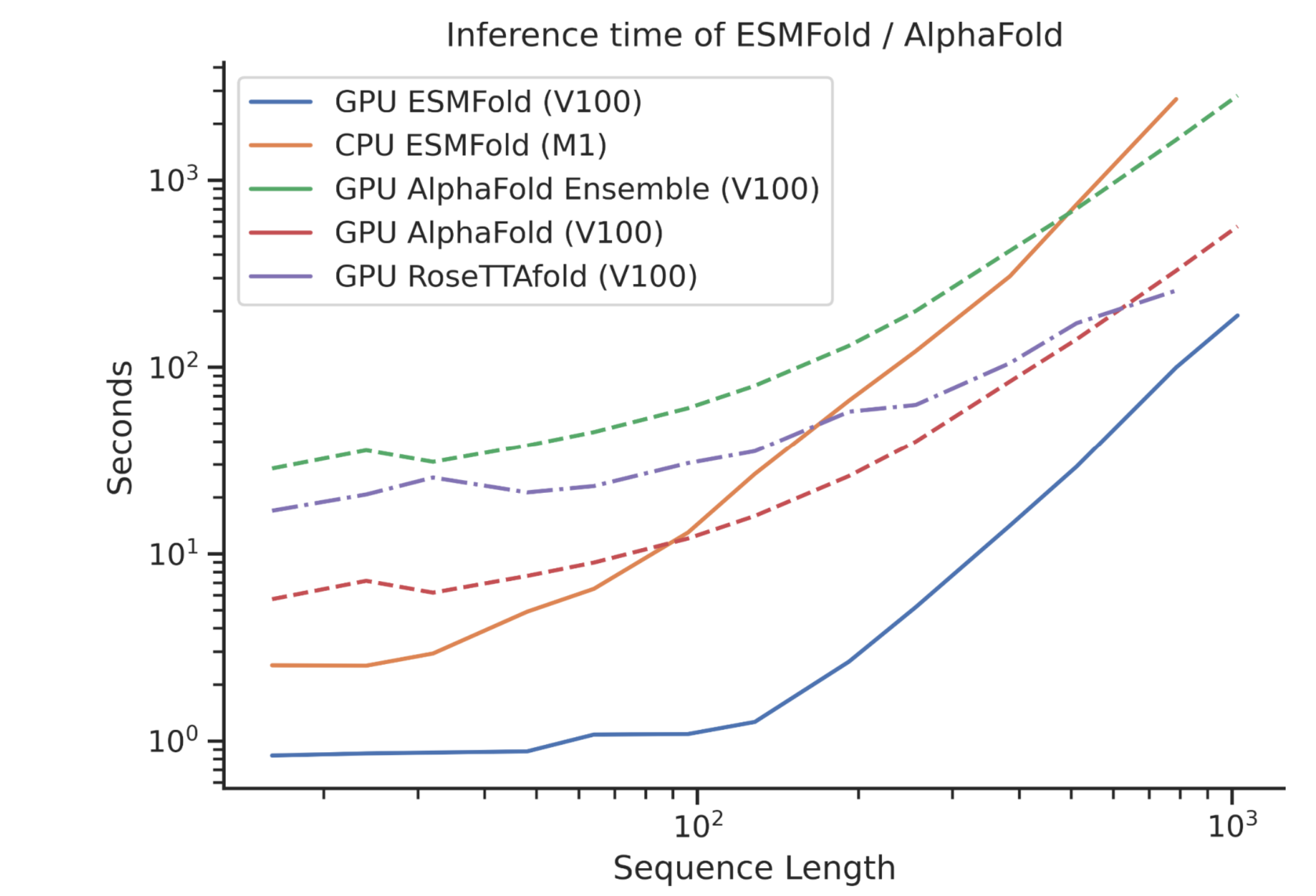
- ESMFold outperforms both RoseTTAFold and AlphaFold2 when given a single sequence as input, and is competitive with RoseTTAFold even when given full MSAs on CAMEO. Scatter-plots show ESMFold against AlphaFold2 performance, colored by perplexity. Proteins with low perplexity under our model score similarly to AlphaFold2. The ESMFold model also has an order of magnitude faster inference time.
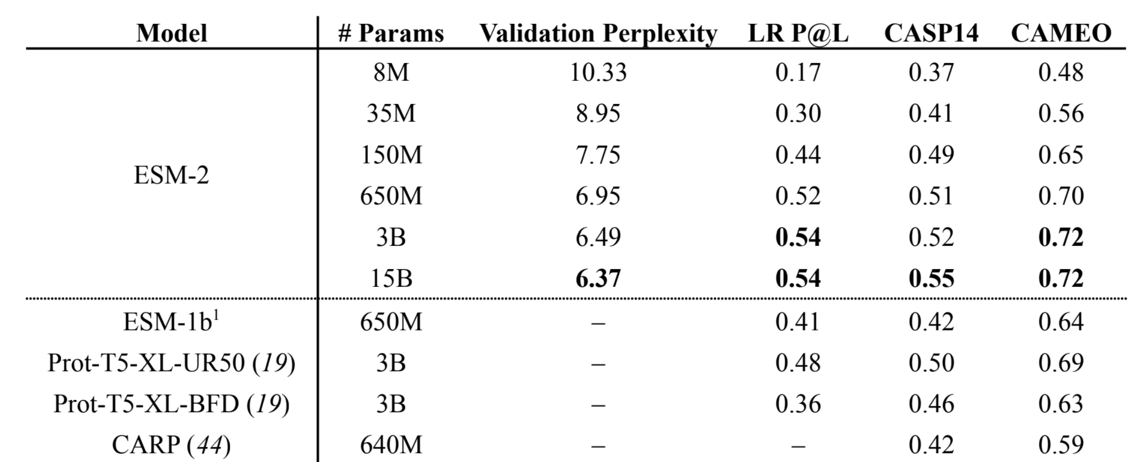
- The 15B parameter ESM-2 model has lowest validation perplexity and highest TM-score on CASP14. The 150M parameter ESM-2 models (and all larger models) outperform the 650M ESM-1b model. The 650M parameter ESM-2 model is comparable with the 3B parameter Prot-T5-XL-UniRef50 model, suggesting


To learn more about protein structure, frame representation (relevant to section 4.1 and 4.2) and Alphafold2, refer to the previous blog post: https://shilpa-ananth.github.io/2025-05-25-Alphafold-2-summary/
Section 4.2: ESM3 architecture and training details
ESM3 is a multiodal masked language model that reasons over the sequences, structures, and functions of proteins each represented as token tracks in the input and output. It was trained on 2.78 billion proteins and 771 billion unique tokens, and has 98 billion parameters. ESM3 is responsive to complex combinations of prompts in sequence structure or function. [10]

Section 4.2.1 ESM3 Tokenization for sequence, structure and function


- Tokenizing Protein sequences: Proteins are tokenized as the 20 canonical amino acids per-residue.
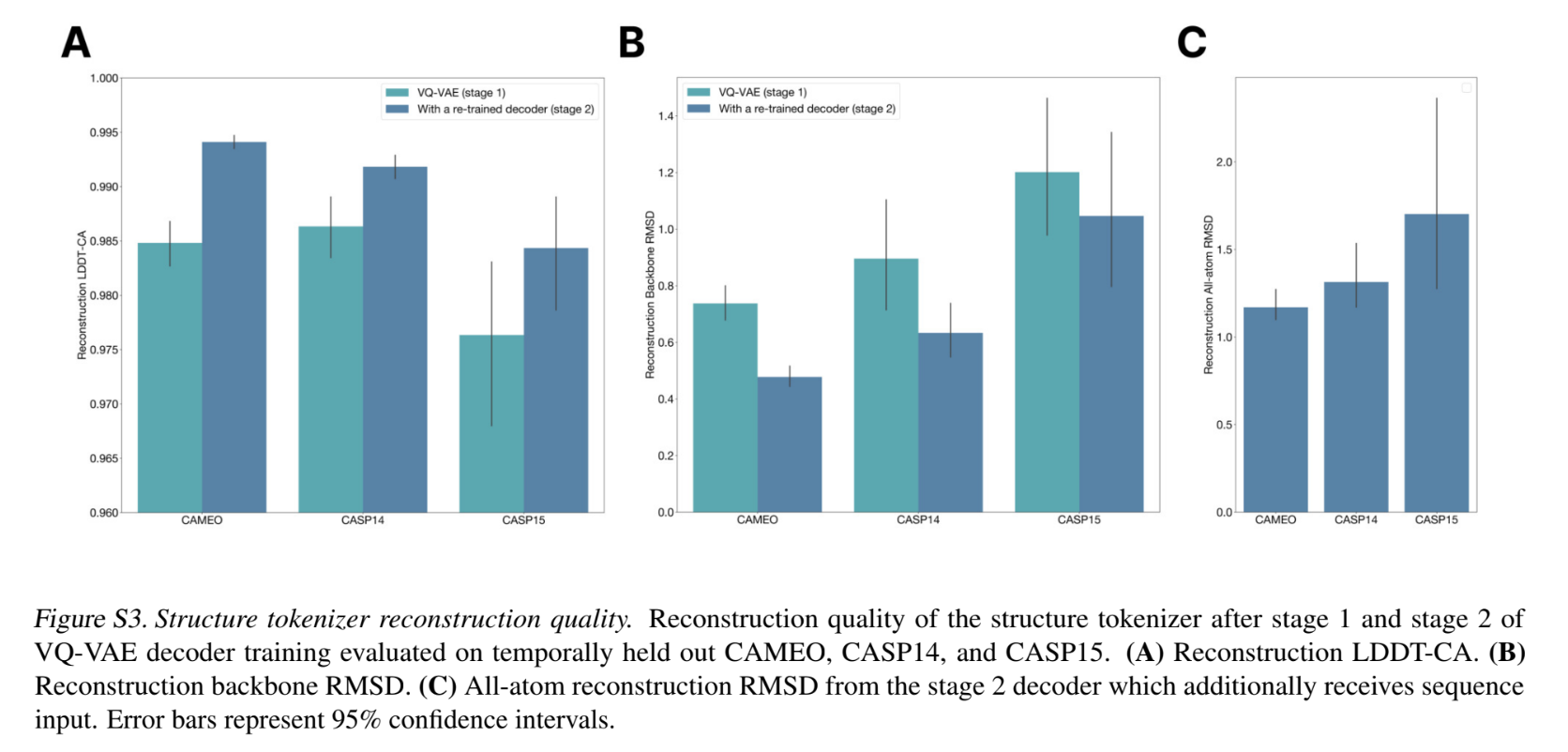
- Structure tokenization: The local structural neighborhoods around each amino acid are encoded into a sequence of discrete tokens, one for each amino acid. The amino acid residues’ 3D structure is tokenized into 4096 discrete structure tokens that provide a representation of the neighbourhood of each amino acid. The structure tokenizer is a VQ-VAE based encoder & decoder, which is trained separately.
- We begin with the co-ordinate location of the C-α carbon atom for each residue, . For each residue, the indices of the 16 nearest neighbours (in the euclidian space, not sequence) are obtained → of size , with the first element being the residue itself. Additionally, the frames for these residues are also obtained.
- The distance of these closest euclidian neighbours mapped to the sequence space is clamped to 32, and embedded embed(). This along with the frames is passed through the VQ-VAE encoder with two geometric attention transformer blocks (more later), with a width of 1024 and 128 heads. The output . The first element for each residue is projected linearly (), and quantized based on a learned codebook () values in [0, 4095].
- Decoder: In the first stage, a smaller decoder trunk consisting of 8 Transformer blocks (with regular attention) with width 1024, rotary positional embeddings, and MLPs is trained to only predict backbone coordinates → Regress a translation vector , and two other vectors that define the plane, these are converted using the gram-schmidt process into backbone frames . In the second stage, the decoder
weights are re-initialized and the network size is expanded to 30 layers, each with an embedding dimension of 1280 (∼600M parameters) to predict all atom coordinates. The side chain torsion angles are also predicted as sine and cosine components which are converted to frames, and back to co-ordinates.
- Five losses are used to supervise stage-1 of training. (a) The geometric backbone distance loss: Constructs the pairwise distance matrix for the predicted and true atom co-ordinates of backbone atoms, and takes their L2 distance. (b) The geometric backbone direction losses: 6 directional vectors are predicted for both the predicted backbone and groundtruth backbone co-ordinates. The pairwise dot product of all these vectors for all residue locations are computed for the predicted and groundtruth vectors, and the L2 loss is computed between the two pairwise matrices. (c) Binned distance and (d) Binned direction classification losses are used to bootstrap structure prediction (e) Inverse folding loss: the final layer representations are used to regress the actual residue values and the cross entropy loss for this task is predicted, this is used as an auxiliary loss.
- In the second stage, the encoder and codebook are frozen, and a deeper decoder is trained to predict all atom co-ordinates (as opposed to just backbone atoms), and incorporate pAE and pLDDT. (a) All atom distance losses and (b) All atom pairwise losses similar to (a) and (b) in point 2d above, extended to all atoms. (c) pLDDT Head and (d) A pAE head to regress specific losses.
- This tokenization delivers near perfect reconstruction of protein structure (<0.5A ̊ RMSD on CAMEO)

- Secondary structure of the protein is represented as 8-class tokens per residue.
- Solvent Accessible Surface Area (SASA) values (usually continuous) are represented as 16 discrete bins
- Function tokenization: Function tokens are a dense semantic representation of functional characteristics of proteins derived from free-text descriptions of the InterPro and Gene Ontology (GO) terms at each residue.
- This free-text is parsed into a count vector for a 68k vocabulary with common unigrams and bigrams. For each residue, all the TF-IDF vectors are max-pooled to get a per-residue annotation. These per-residue vectors are then converted into tokens using 8 locality sensitive hashes each with 8 hyperplanes. The result is a sequence of 8 tokens each ranging in value from 0 to 255 per-residue.
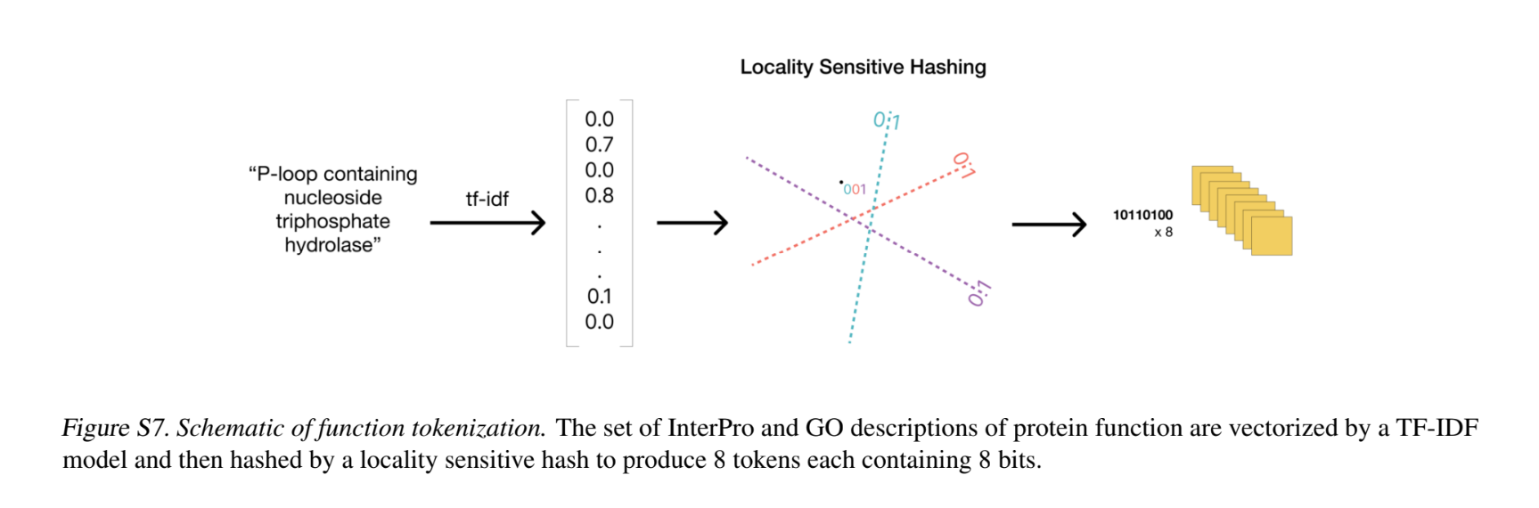
- During pre-training for ESM-3, all 8 tokens of certain residue positions are masked; additionally, corrupted versions of the input tokens are produced by dropping keywords pre-tokenization to change the input tokens. ESM3 is trained to predict the uncorrupted values of all 8 function tokens, each spanning 256 possible values.
- Since the function tokenization with the LSH is a non-invertible process, authors train a 3-layer transformer model to learn the inverse map of the function tokenization process. It is trained to predict the presence of function keywords directly, and the decoder is trained offline separately.

- Residue annotations: Residue annotations label a protein’s sites of functional residues with a vocabulary of 1474 multi-hot labels emitted by InterProScan. At each position there is an unordered set of tokens representing the residue annotations present at that position. The tokens are input to ESM3 first through an embedding lookup followed by a sum over embeddings.
Section 4.2.2 ESM3 Transformer and Geometric Attention
ESM-3 is a “bidirectional” transformer where sequence, structure, and function tokens are embedded and fused at the input, then processed through a stack of transformer blocks. The transformer uses pre layer-normalization. RoPE for positional encodings, and ReLU is replaced with SwiGLU. In accordance with PALM, no biases are used in linear layers. Geometric attention is added to condition on 3D atom co-ordinates in the first layer.
The network consumes positional information in 2 ways (a) The structure tokens (4.1.1) contain information about local neighbourhoods, the authors include a way to directly condition on backbone atomic co-ordinates (b) An invariant geometric attention mechanism to efficiently process three-dimensional structure.
Geometric attention is an SE(3) all-to-all invariant attention mechanism.
- Amino acid residues as frames: The mechanism operates in local reference “frames” defined by the bond geometry at each amino acid residue, and allows local frames to interact globally through a transformation into the global frame. Each local frame consists of a Rotation matrix and a translation vector , and is used to transform a point (relative to the residue i) to the global frame. The “local frame” considers the xy plane such that it spans the N − Cα − C plane, and Cα to be the origin. This is more useful than atom positions, because the model understands how each residue is oriented and positioned relative to its neighbors. Given the global co-ordinates of the 3 backbone atoms, the local “frame” can be determined by the gram-schmidt optimization process.
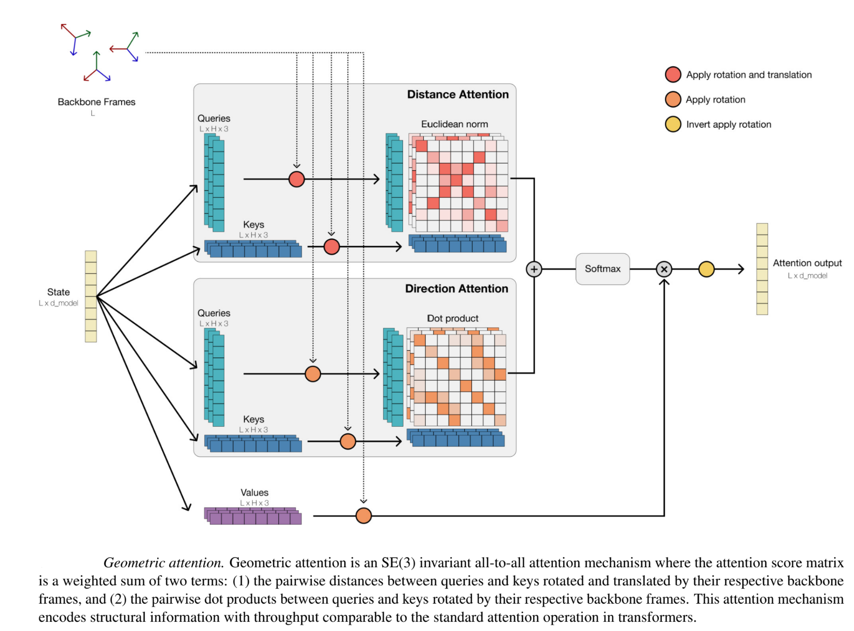

- Geometric attention procedure step-by step: Geometric attention incorporates the frames into the amino-acid embeddings in a rotation/translation invariant way.
- Two sets of keys and queries ( ) and (), along with V, all with shapes ∈ L×h×3 are linearly projected from layer input X. Each of the queries, keys and values are initially assumed to be in the local frame of their corresponding residue.
- Each of the vectors in are converted from their local frame to their global frame by applying from residue i. The pairwise, per-head h rotational similarity R between keys and queries is calculated using the dot product → This is equivalent to encoding the cosine distance between these points.
- Each of the vectors in is converted from their local frame to a global frame by applying . The pairwise, per-head h distance similarity D between keys and queries is computed using the L2 norm of the difference
- These values are weighted and summed, applied to the values vector to form the attention output. In the Geometric Self-Attention layer of ESM3, partially or fully masked coordinates can be input. Undefined coordinates are handled by masking keys and zeroing the attention output wherever coordinates are missing.
Section 4.2.3 Training Procedure and Inference
ESM3 Model training ESM3 are trainec at models at three scales: 1.4 billion, 7 billion, and 98 billion parameters. All the input information is fused into a single representation and processed by the model’s transformer layers. The model is trained for the masked language modelling objective for all tracks simultaneously. At the output of the model, shallow multi-layer perceptron (MLP) heads project the final layer representation into token probabilities for each of the tracks.
- The largest ESM3 model is trained on 2.78 billion natural proteins collected from sequence and structure databases (UniRef, MGnify, PDB, JGI, OAS). The authors also leverage predicted structures from Alphafold anf ESMFold. To leverage this intelligently, ESM3 also uses as input during pre-training — the per residue pLDDT (1 for groundtruth structures, predicted pLDDT from predicted structures) as embeddings, to allow the model to distinguish perfect structures & computationally predicted ones. At inference-time, this value is set to 1.
- As data augmentation during training, the authors also train a 200M parameter inverse folding model, trained on the sequence and structure pairs in PDB, AlphaFold-DB, and ESMAtlas, with the task of predicting sequence at the output given structure at the input. This is used to generate additional sequences corresponding to each structure in the training data for ESM3 (5 sequences per structure for ESMAtlas and AlphaFold-DB, 64 sequences per structure for the PDB).
- During training, a mask for the input tokens is sampled using a noise schedule that varies the fraction of positions that are masked so that ESM3 sees many different combinations of masked sequence, structure, and function, and predicts completions of any combination of the modalities from any other. This supervision factorizes the probability distribution over all possible predictions of the next token given any combination of previous tokens, ensuring that tokens can be generated in any order from any starting point. ESM3’s training objective is also effective for representation learning. High masking rates improve the generative capability, while lower masking rates improve representation learning.
ESM3 Iterative Decoding Since ESM3 is a masked language model based transformer, it can generate samples using any combination of sequence, structure, function prompts. The usual inference strategy is to fix a prompt (full or partial combination of any or all tracks) and choose a track for generation. For predicting the tokens for the generation track, we can perform
- Argmax decoding, which predicts all tokens in the generation track in a single forward pass of the model; runs in O() time in the length of the protein.
- Iterative decoding, on the other hand, samples tokens one position at a time, conditioning subsequent predictions on those already sampled. The runtime for iterative decoding is O(L3) in the length of the protein. When using iterative decoding, choosing the next position to decode can be done by choosing the position with lowest entropy or highest probability. As an in between, we can choose to generate k tokens in one pass.

Section 4.3: ESM3 Results and Outcomes
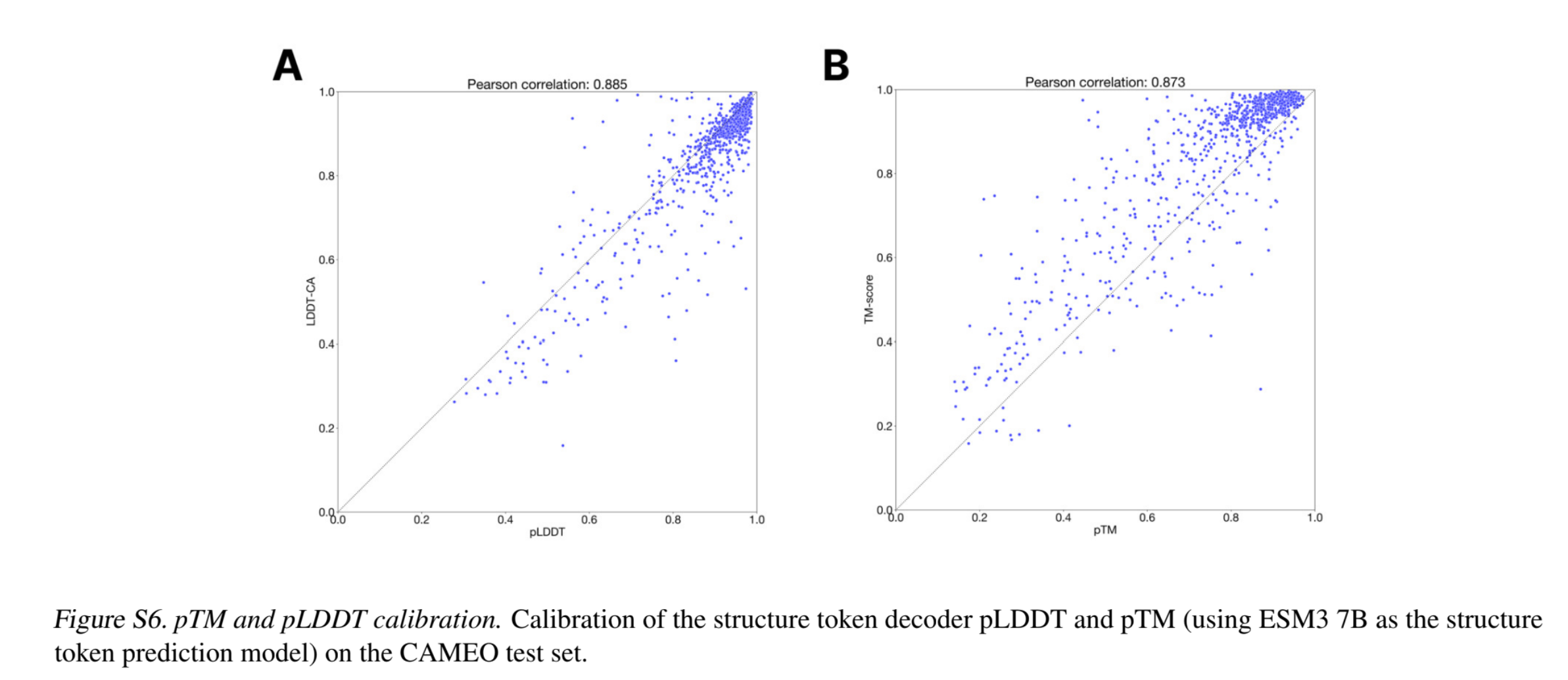
- Zero-shot structure prediction: The pre-trained model can be used directly for structure prediction - to generate the 3D structure co-ordinates, given the sequence. Note that the pTM scores seem to be a slightly under-confident measure and the pLDDT seems to be a sightly over-confident measure.
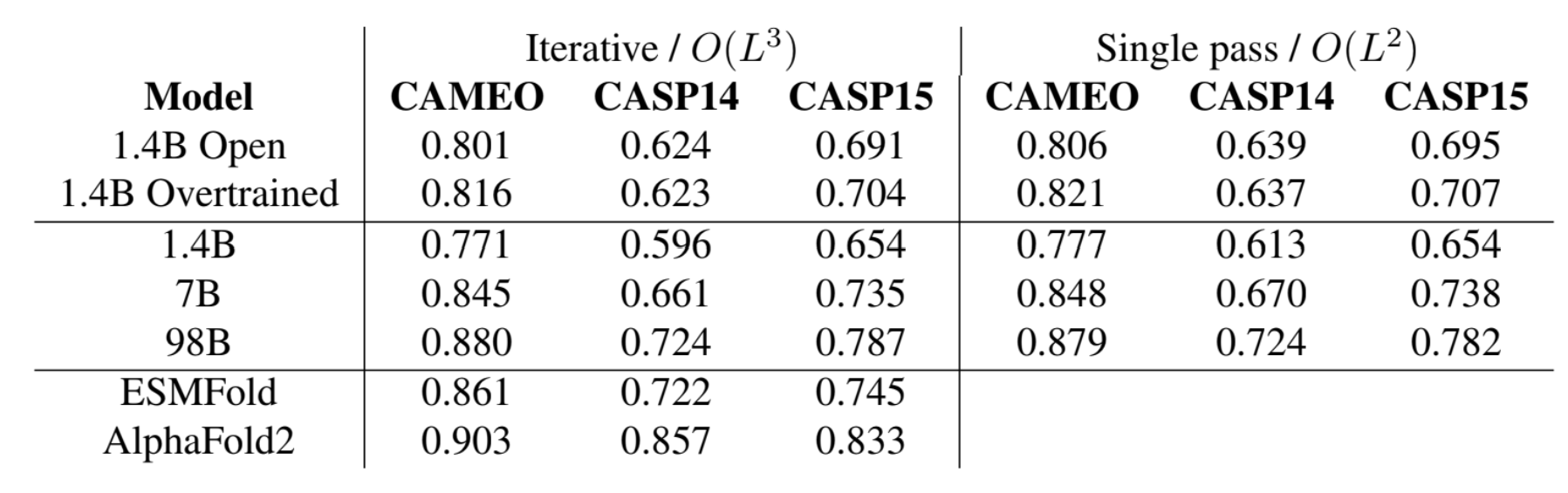


- Representation learning: For contact prediction, an MLP head is added that operates independently over the representations of each amino acid pair, emitting the probability of contact between them. This MLP along with the model is fine-tuned using LoRA adapters for contact prediction. The smallest ESM3 model, with 1.4B parameters, achieves a P@L of 0.76 ± 0.02 on the CAMEO test set, which is higher than the 3B parameter ESM2 model (0.75 ± 0.02), with leser training steps.
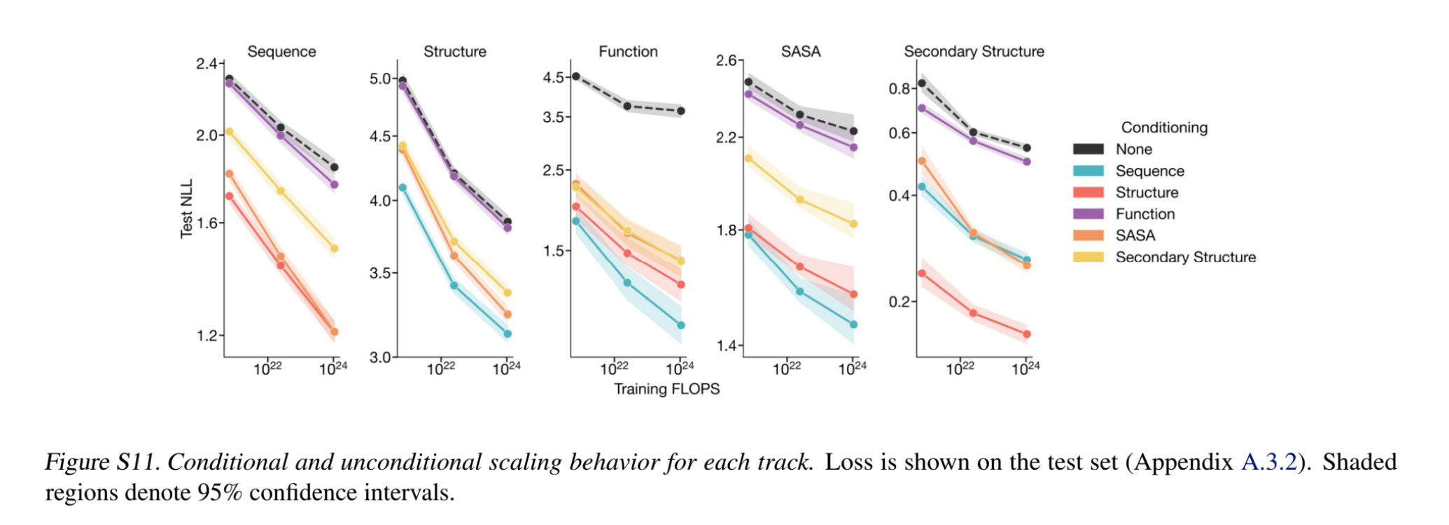
- Conditional likelihood: Given a set of prompts, conditional likelihood of the generations serves as a confidence measure or a proxy for the generative capabilities of the model. Shown below is the negative log likelihood of generating each track, conditioned on other tracks (i.e., given other tracks as input) — adding a conditioning always has a better (lower) negative log likelihood. Note interestingly, that conditioning on sequence results in a lower structure prediction loss than conditioning on secondary structure

- Unconditional Generation of proteins: The authors create a large dataset of model unconditional generations, by sampling 100 protein lengths randomly from the PDB and generating 1,024 sequences for each length. Generating sequences from the model without prompting (unconditional generation) produces high quality proteins—with a mean predicted LDDT (pLDDT) 0.84 and predicted template modeling score (pTM) 0.52—that are diverse in both sequence (mean pairwise sequence identity 0.155) and structure (mean pairwise TM score 0.48)
By using the generated sequences (only) as input, they obtain the model sequence embeddings, and create a protein-level embeddings by averaging over all positions. A sequence ‘similarity’ to the training set was also computed using mmseqs2. Proteins generated unconditionally are similar, but
not identical to proteins found in the training set, without exhibiting mode collapse.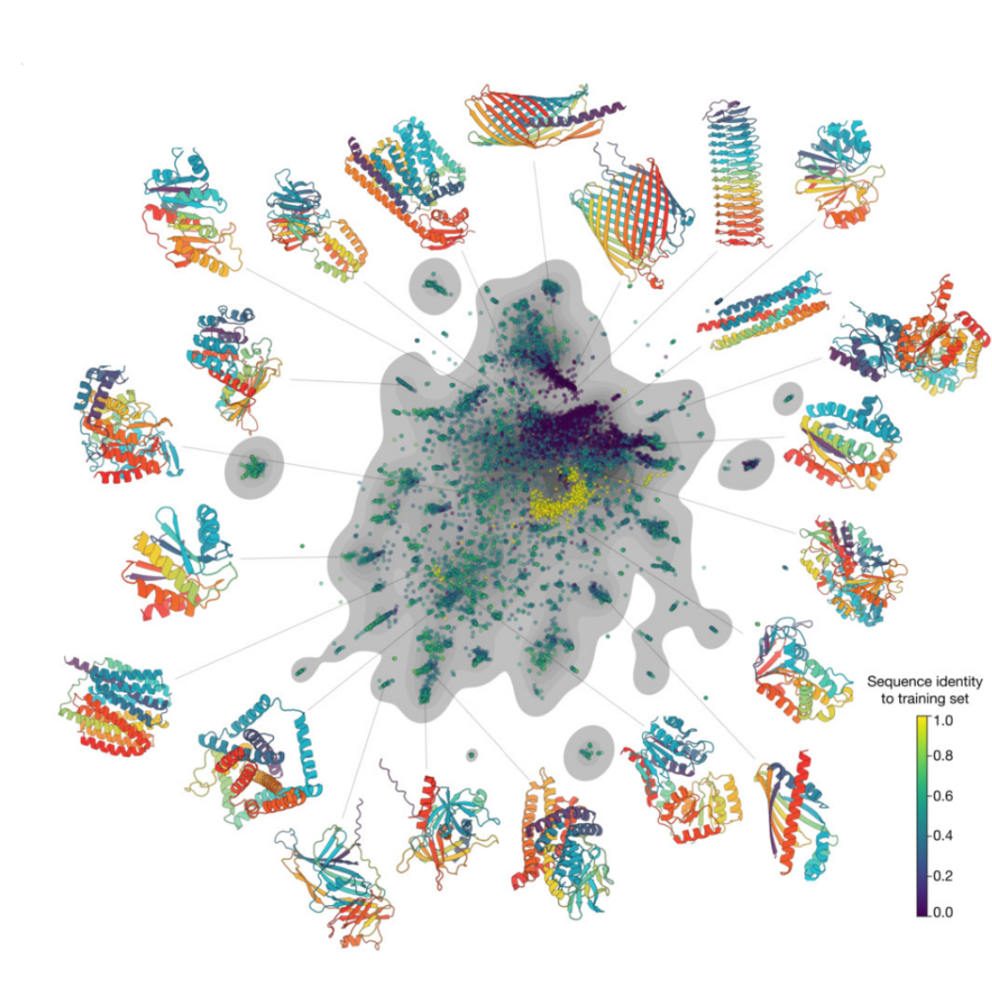

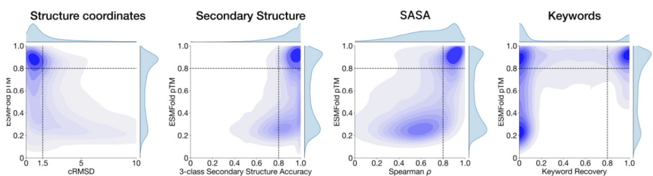
- Ability to follow prompts: A set of prompts are constructed for each of the tracks using a temporally held out test set of natural proteins. The resulting generations are evaluated using ESMFold for consistency with the prompt and confidence of structure prediction (pTM). Consistency metrics include (a) Constrained RMSD — the RMSD between the coordinates of the prompt, i.e. the positions of the backbone atoms, and the corresponding coordinates in the generation; (b) SS3 accuracy, the fraction of residues where three-class secondary structure between the prompt and generations match; (c) SASA Spearman ρ, the correlation between the SASA prompt and the corresponding region of the generation; (d) keyword recovery, the fraction of prompt keywords recovered by InterProScan. Across all tracks, the 7B parameter ESM3 finds solutions that follow the prompt with pTM > 0.8. However, some mode switching is observed in the keyword recovery measure.

- Ability to follow OOD prompts: When using prompts from a set of held-out SS8 + SASA structures, the model continues to generate coherent globular structures (mean pTM 0.85), the distribution of similarities to the training set measured by sequence similarity shifts to be more novel (avg sequence identity <20% to train set)
- Ability to follow complex prompts: The authors prompt ESM3 with motifs that require solving for spatial coordination of individual atoms, including atoms participating in tertiary contacts between residues far apart in the sequence (Eg: catalytic centres / ligand binding). The authors combine atomic-level motif prompts with keywords and generate proteins until there is a success. ESM-3 is able to solve a wide variety of such tasks. Solutions differ from the scaffolds where the motif prompt was derived (median TM-score 0.36 ± 0.14), and for many motifs, there is no significant similarity to other proteins that contain the same motif.
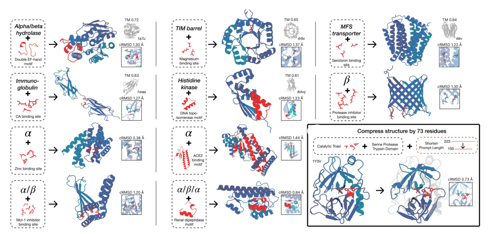

- Biological alignment for complex tasks: Here, the model is aligned to the generative task to satisfy challenging prompts with finetuning. Multiple protein sequences are generated for each prompt and the sequences are folded with ESM3, scoring for consistency with the prompt (backbone cRMSD) and structure prediction confidence (pTM). High quality samples are paired with low quality samples for the same prompt to construct a preference dataset, and ESM3 is then finetuned with a preference optimization loss. After ‘alignment’ to the task, the ability to generate high quality scaffolds (pTM > 0.8) that follow the prompt with high resolution (backbone cRMSD < 1.5 ̊A) is evaluated. Aligned models solve double the tertiary coordination tasks compared to base models. While the base models show differences in the percentage of tasks solved, a much larger capability difference is revealed through alignment. Preference-tuned models not only solve a greater proportion of tasks, but also find a greater number of solutions per task. These results represent state-of-the-art motif scaffolding performance. Compared to a supervised finetuning baseline, which only maximizes the likelihood of the positive examples, preference tuning leads to larger improvements at all scales. The largest aligned model improves substantially relative to the base model before alignment, as well as in comparison to the smaller models after alignment.
- ESM3 generates a biologically functional fluorescent protein:
- Proteins in the GFP family are unique in their ability to form a fluorescent chromophore without cofactors or substrates. In all GFPs, an autocatalytic process forms the chromophore from three key amino acids in the core of the protein. The unique structure of GFP, a kinked central alpha helix surrounded by an eleven stranded beta barrel with inward-facing coordinating residues, enables this reaction. The chromophore must not just absorb light but also emit it in order to be fluorescent.
- The authors directly prompt the base pretrained 7B parameter ESM3 to generate a 229 residue GFP protein conditioned on (a) The positions which are critical residues for forming and catalyzing the chromophore reaction (b) The structure of residues 58 through 71 known to be structurally important for the energetic favorability of chromophore formation. Generation begins from a nearly completely masked array of tokens corresponding to 229 residues, except for the token positions used for conditioning. Generate designs using a chain-of-thought procedure. The model first generates structure tokens, effectively creating a protein backbone. Backbones that have sufficiently good atomic coordination of the active site but differentiated overall structure from the 1QY3 backbone pass through a filter to the next step of the chain. Add the generated structure to the original prompt to generate a sequence conditioned on the new prompt. Then perform an iterative joint optimization, alternating between optimizing the sequence and the structure.
- The computational pool of tens of thousands of candidate GFP designs are bucketed by sequence similarity to known fluorescent proteins and filtered and ranked using a variety of metrics. The top generations in each sequence similarity bucket are synthesized, expressed in E. coli, and measured for fluorescence activity at an excitation wavelength of 485 nm. Brightness similar to positive controls was measured from a number of designs that have higher sequence identity with naturally occurring GFP. The authors identify a design with only 36% sequence identity to the 1QY3 sequence and 57% sequence identity to the nearest existing fluorescent protein, tagRFP. The chain of thought is continued from the sequence to generate a protein with improved brightness.
- The best design is designated as esmGFP and exhibits brightness in the distribution of natural GFPs. A BLAST search against the non-redundant protein sequences database and an MMseqs search of ESM3’s training set report the same top hit—tagRFP, which was also the nearest neighbor to B8—with 58% sequence identity, representing 96 mutations throughout the sequence, which is estimated to be over 500 million years of evolution close to esmGFP.
[1] The Cell: A Molecular Approach, 8th edition
[2] Sequence modeling and design from molecular to genome scale with Evo | Link and Supplementary Info: (🔗Science) (🔗 bioRxiv)
[3] 🔗 MLCB Lectures – Protein Language Models (MIT)
[4] 🔗 Genome Engineering Using the CRISPR-Cas9 System (Nature)
[5] 🔗 CRISPR-Cas9 Mechanism – YouTube Video
[6] 🔗 Nature Video: CRISPR — Gene Editing and Beyond
[7] 🔗 CRISPR Deep Dive – YouTube
[8] ESM-1: Biological Structure and Function from Unsupervised Learning at Scale
[9] ESM-2 and ESMFold: Language Models Enable Accurate Structure Prediction
[10] ESM-3: Simulating 500 Million Years of Evolution with a Language Model