Alphafold - A Technical Summary

Section 1: Preliminary information

Proteins are polypeptides of amino-acids: Proteins direct virtually all activities of the cell and have a wide variety of functions (information transmission, chemical reaction catalysis, cellular transport, infection defense, etc.). Proteins are polymers synthesized from 20 different amino acids. Each amino acid consists of a carbon atom (called the α carbon) bonded to a carboxyl group (COO–), an amino group (NH3+), a hydrogen atom, and a distinctive side chain — the side chains determine the chemical properties of the amino acid, and contribute to the overall structure and function of the protein. [1] Amino acids are joined together by peptide covalent bonds between the α carboxyl group of one amino acid and the α amino group of a second. Polypeptides are linear chains of amino acids, usually hundreds or thousands of amino acids in length. Each polypeptide chain has two distinct ends, one terminating in an amino group (the amino, or N, terminus) and the other in a carboxyl group (carboxy, or C, terminus).

Amino acids and the protein structure: The amino acid sequence eventually determines the protein’s 3D shape; the chemistry of the side chains is critical to protein structure because these side chains can bond with one another to hold a length of protein in a certain shape or conformation by nature of their properties — charges (leading to ionic bonds), polarity (leading to hydrogen bonds), hydrophobic nature (leading to Van der Waals forces). Although these side chain interactions are largely non-covalent, they are strong enough to guide where the bends and folds and rotations occur in that protein. [2] There are 4 levels of organization of protein structure (a) The protein primary structure is considered it’s amino acid sequence. (b) Its secondary structure refers to the local arrangements of the chain in space — common examples include alpha helix and beta sheets (c) The tertiary structure is its overall three-dimensional shape, once all the secondary structure elements have folded together among each other (b) The quatenary structure is the assembly of multiple polypeptide chain sub-units interacting with each other. [3]

Challenges and common methods of Protein Structure Prediction: The C-N bond (peptide bond) has a partial double bond character and remains relatively fixed; this angle ($\Omega$) is usually 180 and has little significance in polypeptide folding. There are two essential torsion (rotation) angles in the polypeptide chain, also called Ramachandran angles. These angles describe the rotations of the polypeptide backbone around the bonds between N-Cα (called Phi, φ) and Cα-C (called Psi, ψ) and essentially determine the fold of the protein (more on torsion angles and side chain angles later). The protein folding problem is highly challenging because of the sheer number of possible conformations of the φ and ψ of each monomer of the polypeptide chain. Older methods of modelling the physical interactions using thermodynamic or molecular stimulations tend to be computationally intractible. Other current methods include analysis of pairwise evolutionary correlations and homology (~similarity) with solved proteined structures, however, these fall short on level of accuracy required for widespread adoption and utility.

Section 2: Enter Alphafold2!

Alphafold2’s neural network architectures and training procedure led to a greatly improved 3D structure prediction in the CASP14 challenge, beating the next best solution by a large margin[4]. The rest of the article is a step-by-step overview of Alphafold2, based on the paper and the supplementary section, as well as several fantastic blogs referenced below. [5][6][7]

Section 2.1 Inputs and Processing

2.1.1 Primary Input Data Sources

The models were trained on the PDB (ProteinDataBank) database that contains protein sequences and their groundtruth protein structures. The inputs to the network during training are —

1. The primary protein sequence from Protein Data Bank (input) and 3D atom co-ordinates of homologous sequences from Protein Data Bank (label)

2. Genetic search for Multiple Sequence Alignments: For each train sequence a Multiple sequence alignment (MSA) with evolutionarily related (homologous) proteins is fetched. Intuitively, MSAs help deduce information about protein structure — for example, if mutations observed at two points (sequentially far away from each other) are highly correlated, chances are they’re actually physically close to one another when folded. This is explained well here. To find the MSA structures at train time, tools like JackHMMER and HHBlits (tools for accurate distant homology detection) are used on large databases like Uniref90, BFD, Uniclust30, and MGnify. The output MSA’s are de-duplicated and stacked. The depth and diversity of MSAs significantly impact AlphaFold’s ability to infer residue interactions and folding patterns.

3. Structural templates AlphaFold uses the Uniref MSA (above) to search PDB70 (a curated subset of PDB) using HHSearch to find homologous structures’ 3D atom co-ordinates ( along with residue interactions, and secondary structure annotations). This information fed as input to the network could help it deduce similar structures from highly related protein sequences. Note: During training, All template structures released after the primary input sequence are dropped, and templates that are too small are dropped.

2.1.2 Pre-pocessing the sequences during training

MSA features and pre-processing — Some data augmentation and space optimisation techniques are used to modify the MSA features:

1. MSA Block deletion: During training contiguous blocks of sequences are deleted from the MSA, to generate diversity that removes whole branches of the phylogeny.

2. MSA Clustering: The aim here is to reduce the number of sequences in the MSA ($N_{seq}$) to ~128 ($N_{clust}$). First, a set of random $N_{clust}$ sequences are selected as representatives. The remaining sequences are matched with their ‘nearest’ representative sequence, and used to generate a mini sequence profile. This profile is fed along with each representative sequence as input to the network so that all sequences not included still influence the final prediction.

3. MSA masking: 15% of the amino acids in each cluster centre are masked — at each masking position, the amino acid is either (i) Replaced with a masking token (ii) Replaced with an amino acid at random, or sampled from the mini sequence profile distribution at that position.

4. The residues dimension is cropped to a single contiguous region, and the final crop size is denoted by $N_{res}$.

Template features and pre-processing —

1. A Template distogram is created for the template structures. This is a one-hot pairwise feature indicating the pairwise distance between every one of the amino acids (beta carbons atoms) in the chain. The distance is binned into 38 intervals.

2. Template torsion angles: The 3 backbone torsion angles and up to 4 side-chain torsion angles for each residue represented as sine and cosine encodings (more details on torsion angles in the structure modules)

Other additional features are listed in supplementary information section 1.2.9 of the Alphafold2 paper.

2.1.3 Input processing: Converting input information into embeddings

1. Creating input embeddings: The primary input sequence (target_feat) is transformed with two linear embeddings and outer-summed to form a pairwise representation [$z_{ij}=a_i+b_j$, where $z_{ij} \in \R^{c_z}$ ] . This is followed by addition with the original sequence converted to a relpos representation, that computes clipped relative positions between amino acids in the chain (equivalent to positional embeddings in sequence models). As a result, we have the initial pair representation of the input sequence $z_{ij}$.
   The MSA features (msa_feat) also go through a linear layer, and added to a transformed represenation of the input sequence to form the initial MSA represenation.
   

2. Integrating information from the templates: Next, template information is incorporated into both these embeddings. The template sequences and the torsionangles (contained in template_angle_feat) are transformed by linear layers and concatenated to the initial MSA representation. The template distogram related features (template_pair_feat) are embedded with a shallow attention network and added to the pairwise representation.

3. Processing extra MSA features: The MSA features not selected as cluster centres ($N_{seq}-N_{clus}$) are processed by a shallow optimised Evoformer network and this is used to update the pairwise representation.

At the end of this processing stage, we have an MSA representation and a pairwise representation, both containing information about the original sequence as well as the template sequences.

Section 2.2: The Evoformer

The Evoformer uses attention-based mechanisms that allows it to dynamically learn interactions between non-neighboring nodes, and focus on computing the graph of how each residue relates to another [8].

Each of the 48 Evoformer blocks in the evoformer stack has an MSA tower and the pairwise representation tower (pictured horizontally below). The MSA representation is processed with axial self attention, and the pairwise representation is processed with triangular updates and triangular self attention. Both representations are also used to update each other. The MSA representation and the pairwise representation pass through the Evoformer stack $N_{cycle}$ times and are updated each time before the next cycle.

2.2.1 The MSA representation updates

The MSA representation undergoes row-wise and column-wise gated self attention, which are forms of axial self attention. Remember that the MSA representation is large because $N_{res}$ i.e., $r$ is huge — so axial attention factorizes the attention computation across the row and column dimension and is more efficient for high dimentional data.

1. Row-wise gated self attention with pair bias: Each row is updated with self attention from all residues within the same row, with a bias from the pairwise representations (to maintain consistency between pairwise and MSA representations). This way, information flow happens between all residues of a single sequence and is used to update each sequence.

2. The column-wise attention lets the elements that belong to the same target residue position exchange information. The column is updated with information from all other residues of the same column.

3. Following this is an MSA transition layer, that expands and compresses the number of channels

2.2.2 Pairwise representation updates

Outer Product Mean: As a first step in this parallel branch, the MSA representation is incorporated into the pairwise representation. To do this, the MSA entries are linearly projected into a small dimension. Then for two ‘columns’ $(i, j) \in 1…r$, the outer products of the vectors at each row are taken and averaged over the sequences. Finally, this matrix is flattened and linearly transformed to form the element at $(i, j)$ of the pairwise representation. This is a neat way of transforming the MSA representation $(s, r, c_m)$ into a similar dimension as the pairwise representation to be incorporate into the existing pairwise representation

Triangular multiplicative updates: The triangle inequality is not enforced in the model but rather, it is encouraged through ensuring each position $z_{ij}$ is updated by looking at all possible triplets of positions (i,j,k) at a time [6][9]. However if we were to anchor on a value k, remember that in the pairwise representation we have both $z_{ik}$ and $z_{jk}$ in the matrix, as well as $z_{ki}$ and $z_{kj}$. Intuitively, apart from just encoding physical distances imagine these pairwise representations to also encode directional influences each residue may have on the other. To account for updates in all possible directions, Alphafold divides updates into two steps, “incoming edges” wrt k and “outgoing edges” wrt k (Figure 4c).

$z_{ij}$ is updated based on $z_{ki}$ and $z_{kj}$ for all other atoms k for the “incoming edges” (incoming to i and j from k) triangular update.

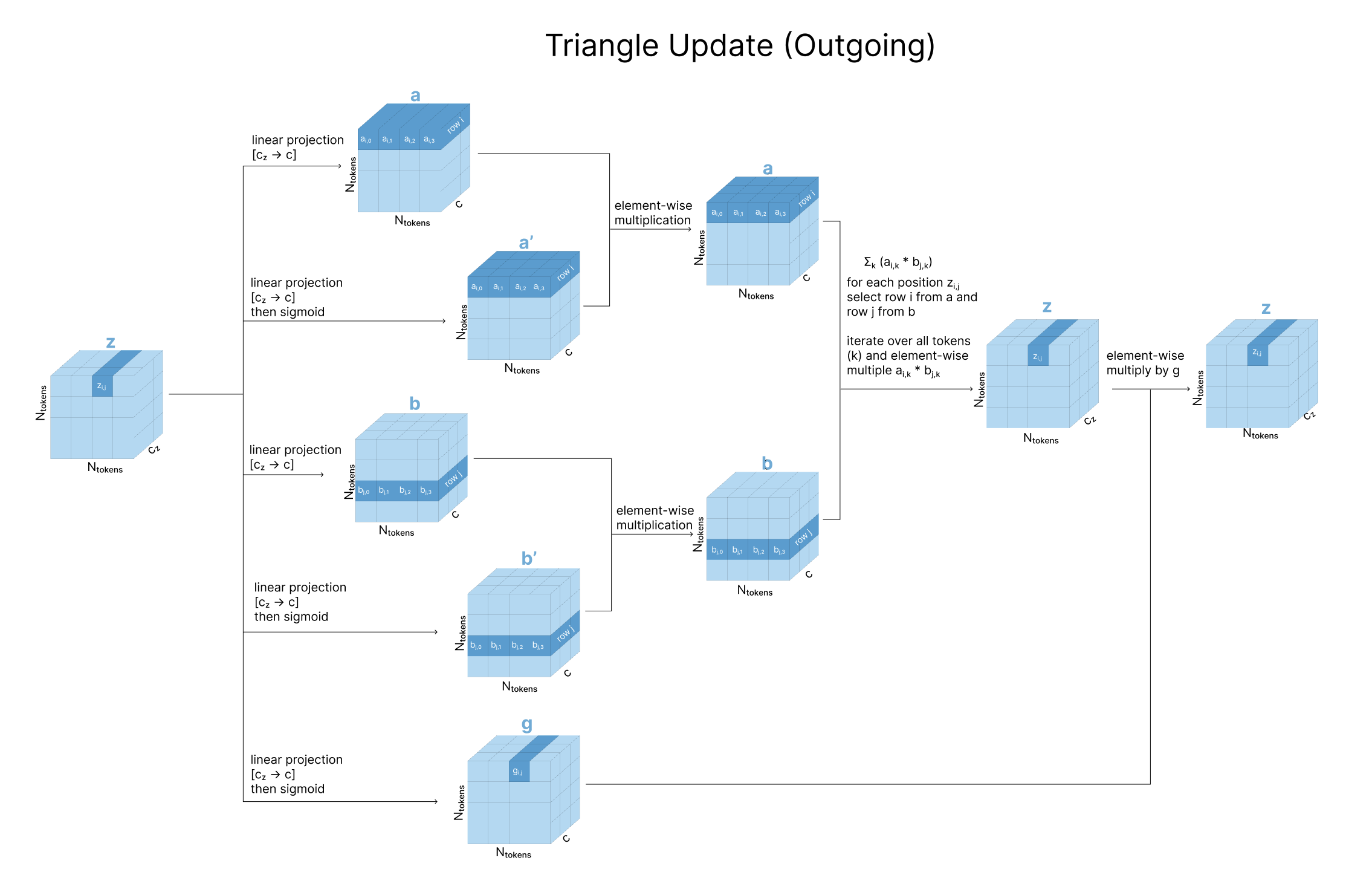
$z_{ij}$ is updated based on $z_{ik}$ and $z_{jk}$ for all other atoms k for the “outgoing edges” triangular update

Triangle attention updates: Triangle attention incorporates the triangle principle to attention, updating $z_{ij}$ by incorporating $z_{ik}$ and $z_{jk}$ for all atoms k.

Starting Node Triangle Attention Specifically, in the “starting node” case to calculate the attention scores for $z_{ij}$ we want to find the influence of all other nodes on node $i$ (that is all $z_{ik}$) biased by the influence node j on those same nodes.

Query $\to z_{ij}$
Keys, values
$\to z_{ik}$ for all values of k

Bias
$\to z_{jk}$ for all values of k (reduced to channel = 1 using linear projection)

Finally, the transition layer for the pairwise representation contains a 2-layer MLP where the intermediate number of channels expands the original number of channels by a factor of 4.

Section 2.3: The Structure Module

2.3.1 Structure module Preliminaries

Alphafold2 was one of the first works to predict the backbone atom positions directly, rather than predict distances or correlations. To do this, the aminoacid residues are represented as a residue gas comprised of “backbone frames” (parametrized by $T_i$) and and “torsion angles” ($\vec{\alpha}^{f}_i$).

• What are “frames” here? Each residue backbone ‘frame’ is defined as the geometry of a triangle of “N (nitrogen) — $C_{\alpha}$ (alpha carbon) — C (carbonyl carbon)” of each residue with respect to the global frame. Each frame is represented as an $T_i = (R_i, \vec{t}_i)$ pair, $\forall i \in (1, ... N_{res})$. Here, $R_i \in 3 \times 3$ is a rotation matrix of the frame and $t_i \in 3 \times 1$. These rotation and translation matrices help compute the location of the ‘frame’ or the rigid body, with respect to the global frame.

Each atom position in an amino acid residue can be determined by backbone torsion angles ($\omega, \phi, \psi$ that signify positions of atoms other than $N$, $C_\alpha$, C) and side chain trosion angles $\chi_1, \chi_2, \chi_3, \chi_4$. (The bond length and bond angle is assumed to be almost always same ). This is represented in the network by $\vec{\alpha}^{f}_i \in \R^2$ where $i \in \{1, ... N_{res}\}$ and $f \in \{ \omega, \phi, \psi, \chi_1, \chi_2, \chi_3, \chi_4 \}$.

As the single representation $s_i$ and the pairwise representation $z_{ij}$ cycles through the structure modules, they are used to update the backbone frames and predict the Torsion angles.

2.3.2 Structure Module Architecture

2.3.3 Invariant Point Attention Module

Alphafold uses a version of the iterative SE(3)-Transformer. The Iterative SE(3)-Transformer is a graph transformer with a customized attention mechanism designed to be equivariant under continuous 3D roto-translations — ie the output remains consistent even when the input is transformed by a global change. In Alphafold2, this mechanism is incorporated in the Invariant point attention — Attention between two residues on 3D space that is invariant to global transformations. The IPA module updates the abstract single representation using multiple “channels” of attention:
(1) It first computes the usual self-attention for the single representation (2) Then it converts the pair representation into a simple element-wise “pair bias” to incorporate into the attention module (3) Next, it converts the backbone frames into “distance affinities”, which can be thought of simply as representing distances. This serves two purposes: the attention between two points is determined based on the distance between the points. Additionally, this attention term is invariant to global transformations

Finally, it adds all of these to obtain a final set of attention weights, which are then combined with vector representations of each input type and summed for the final single representation update.

Any global rotation or translation cancels out in the “distance affinity” term, because the L2-norm of a vector is invariant under rigid transformations.

2.3.4 Structure module outputs

Backbone updates: The updates for the backbone frames are learnt from the (IPA updataed) single sequence representation $s_i$

Torsion angle prediction: The updated single representation is also used to predict the torsion angles $\vec{\alpha}^{f}_i \in \R^2$ where $i \in \{1, ... N_{res}\}$ and $f \in \{ \omega, \phi, \psi, \chi_1, \chi_2, \chi_3, \chi_4 \}$ using a shallow resnet.

Updated single sequence representation $s_i$: The single sequence representation $s_i$ from the Evoformer module, updated by applying IPA in the recursive blocks of the structure module.

2.4 The Final Network Outputs and Losses

The outputs of the network include

1. The Co-ordinates of all residues and their atoms (2.3.4 above)

2. PLDDT head — predicts the per-residue (pairwise) lDDT-C$\alpha$ scores which is the intrinsic model accuracy / uncertainty estimates. This is predicted by taking the final single representation from the structure module, and projecting it into 50 bins (each bin covering a 2 lDDTC$\alpha$ range) and applying softmax. To create targets while training, network uses the final strcture module prediction and computes the lDDT-C$\alpha$ against the groundtruth.

3. TM-score head — Predictor of the global superposition metric TM-score, a more accurate global similarity measure between two protein structures. In alphafold, this value is computed over all possible alignment single residue alignments that can be used to compute the pairwise distance between atoms. The model predicts a modfied term of this error metric by applying a linear layer and softmax over the single representation.

4. Distogram predictions: The pairwise representation $z_{ij}$ from the evoformer output is used to predict a distogram — pairwise matrix representing distance between each set of $\beta$ carbon atoms. The $z_{ij}$ is symmetrised (by summing it with the trasnform) and a linear projection into 64 bins (with softmax) is applied to predict the distogram. The targets are computed from the ground truth atom positions, and converted to one-hot binned values for training.

5. Masked MSA prediction: The final $m_{si}$ representation is also used to predict the masked values from the MSA representation (during pre-processing), similar to an MLM (masked language modelling) objective.

The network is trained with the gradients from the FAPE loss and a number of auxiliary losses.

1. Frame Aligned Point Error (FAPE) Loss: Compares the predicted atom positions to the true positions under many different alignments. The final FAPE loss is computed over all backbone and side chain atoms. The loss between predicted atom position $\vec{x}_j$ relative to frame $T_i$ and true atom position $\vec{x}_{j}^{true}$relative to $T_i^{true}$ is computed as an L2 norm for each atom. For each alignment, defined by aligning the predicted frame $(R_k, t_k)$ to the corresponding true frame, we compute the distance of all predicted atom positions $\textbf{x}_i$ from the true atom positions. The resulting $N_{frames} × N_{atoms}$ distances are penalized with a clamped L1 loss.

2. Torsion angle losses: The side chain and torsion angles are compared with the groundtruth torsion angles with an L2 loss in $\R^2$ (points in a unit circle). This is mathematically equivalent to the raw angle difference.

[1] The Cell: A molecular approach

[2] 🔗 Protein Structure (Nature Scitable)

[3] 🔗 Protein Structure - LibreTexts

[4] 🔗 AlphaFold - DeepMind Blog

[5] 🔗 AlphaFold 2 - Blopig Blog

[6] 🔗 The Illustrated AlphaFold

[7] 🔗 AI4Pharm - AlphaFold2

[8] 🔗 AlphaFold2 Architecture - PIIP

[9] 🔗 AlphaFold2 Video - YouTube