Note: A lot of the content here is based on my learnings from Bishop, lectures by Jeff Miller (highly recommend), and several other resources linked in references below
A graph comprises nodes (also called vertices) connected by links (also known as edges or arcs). In a probabilistic graphical model, each node represents a random variable (or a random vector), and the links express probabilistic relationships between these variables. It captures the way in which the joint distribution over all of the random variables can be decomposed into a product of factors each depending only on a subset of the variables
Section 1: "Bayesian" networks / Directed Graphical models/ and Joint PDFs
“Bayesian” networks are useful tools to visualise the random variables and their relationship as a graph. They are useful because you can (a) Factorization of the probability distribution into conditionals can visualized (b) The conditional independence properties become more evident. Visualizing the models also helps us make simplified inferences by leveraging the conditional independence properties of the graph.
Section 1.1: Graph factorization
Note 1: Shaded random variables indicate conditioning. (these variables are observed). RV's that do not have observed values are often called latent variables or hidden variables.
-
-
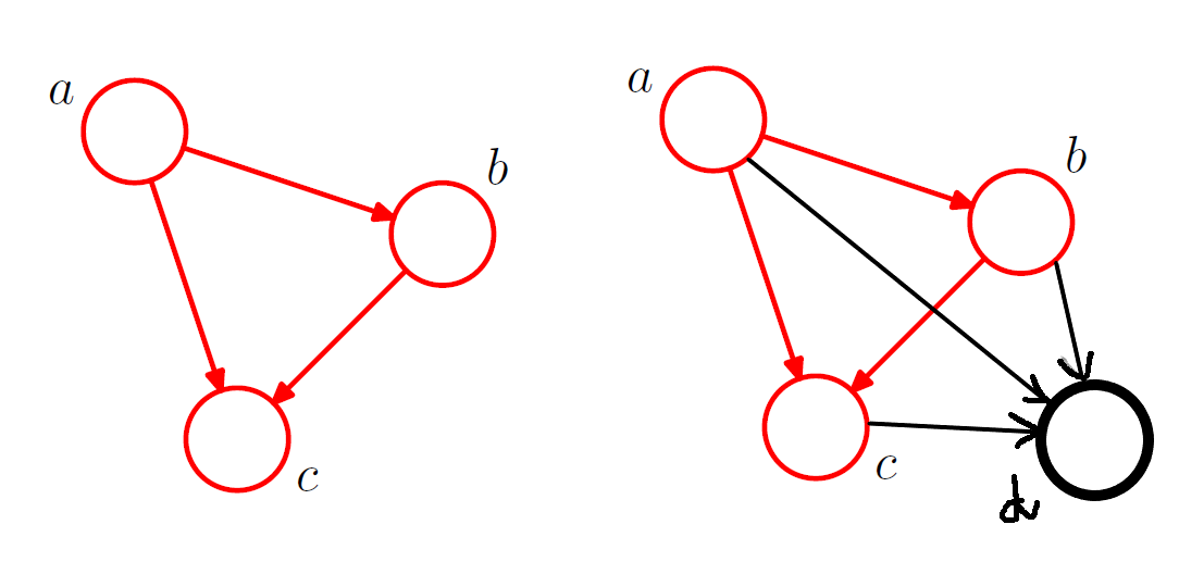
For a fully connected DAG graph with K random variables, we define
In the absence of certain links, the distribution is modified accordingly. For figure 3 on the right above, the joint distribution is given by
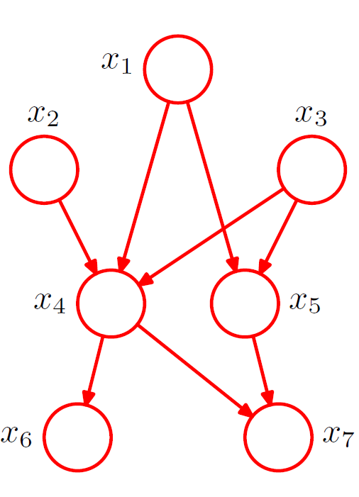
In general, given an ordered DAG on n vertices, the JPDF can be written as subject to constraints that there are no cycles.
Note 2: In the JPDF factorization above, we can also denote the whole JPDF in terms of the JPDF of a sub-graph.
Note 3: For any given graph, the set of distributions that satisfy the graph will include any distributions that have additional independence properties beyond those described by the graph. For instance, a fully factorized distribution will always be passed through the filter implied by any graph over the corresponding set of variables.
Section 1.2: Some Practical Visualization Examples
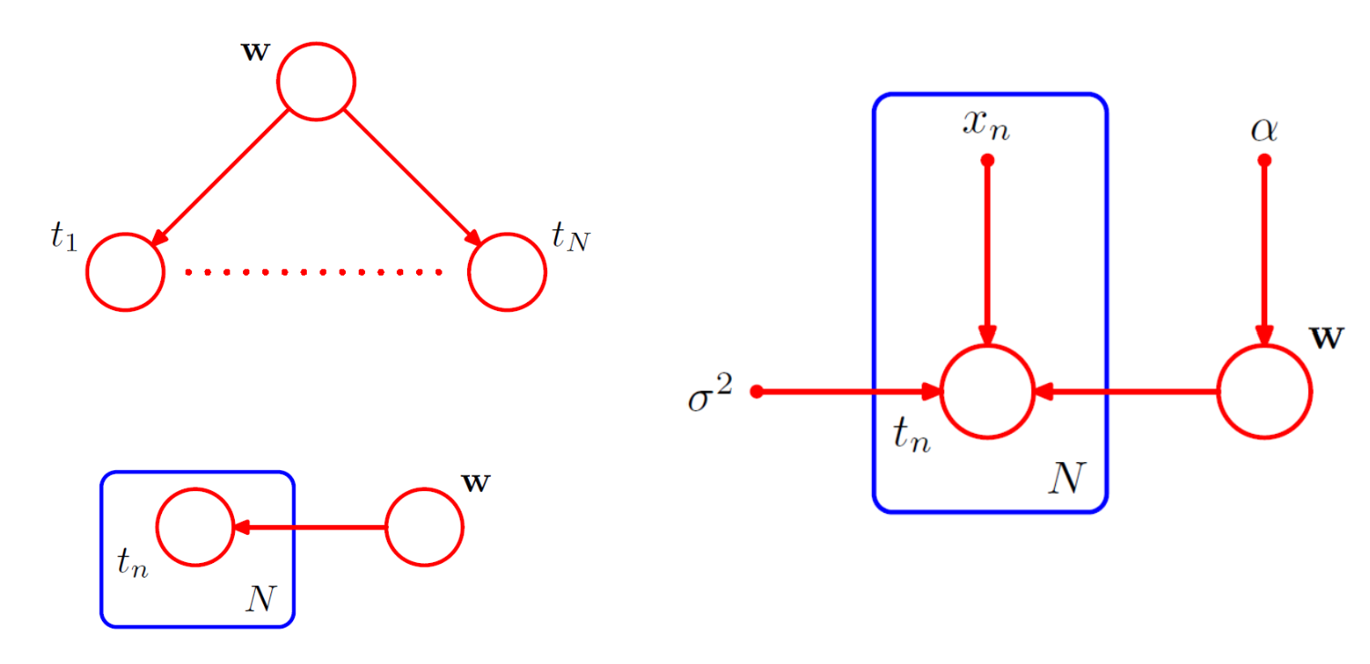
Polynomial regression:
The random variables in this model are the vector of polynomial coefficients and the observed data . In addition, this model contains i.e., the input data, the noise variance , and the hyperparameter α representing the precision of the Gaussian prior over , all of which are parameters of the model rather than random variables.
The figure below shows the simple graph structure of random variables; the plate diagram and the fully descriptive graph structure with the deterministic parameters. The input and parameters are denoted without circles around them. Note that is not a ‘variable’. The repetitive variables are condensed into a ‘plate’
The joint distribution
given the parameters of polynomial regression is given by . Note that the value of is not observed, and so is an example of a latent variable, also known as a hidden variable.
When t values are observed, we can calculate the posterior
proportional to .
Section 1.3: Conditional Independence
Given three nodes of a graphical model a, b, c; a is said to be independent of b given c if it satisfies the following condition and . To interpret conditional independence from graphical models we use a concept called d-separation.
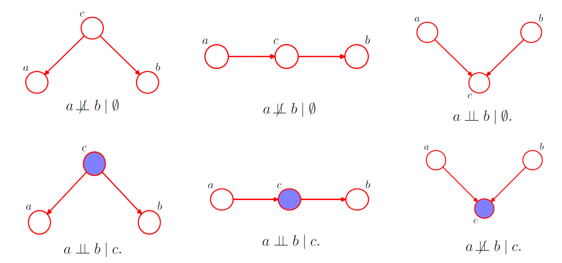
- When the node c between a and b is tail to tail connected; it blocks the path when c is observed, making the variables a and b conditionally independent
- When the node c between a and b is head to tail connected; it blocks the path when c is observed, making the variables a and b conditionally independent
Therefore,
- When the node c between a and b is head to head connected; it opens the path when c is observed, making the variables a and b conditionally dependent
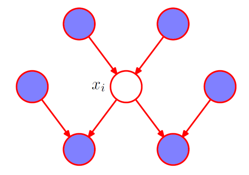
In a DAG, if all the paths from A to B are blocked given C, A is said to be d-separated from B given C, and it satisfies the condition A⊥B | C. The Markov blanket of a node comprises the set of parents, children and co-parents of the node. We can think of the Markov blanket of a node as being the minimal set of nodes that isolates from the rest of the graph. Note that it is not sufficient to include only the parents and children of node because the phenomenon of explaining away means that observations of the child nodes will not block paths to the co-parents.
Section 1.4: d-separation
Consider 3 disjoint set of vertices (A, B, C) in a DAG. A ‘path’ is defined as a set of vertices such that there is an edge between the vertices. The path between A and B is said to be “blocked” wrt if
(a) There exists a head to tail vertex or a tail to tail vertex in that path that belongs to C; or
(b) There exists a head to head vertex in that path where that vertex (and all its descendents) are not in C.
A and B are D-separated by C if all paths between A to B are ‘blocked’ by C; and in this case (i.e., when C is observed)
Section 2: Hidden Markov Models
Section 2.1: Markov chains
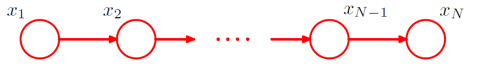
In probability theory and statistics, a Markov chain or Markov process is a stochastic process describing a sequence of events in which the probability of each event depends only on the state attained in the previous event. These Markov Chains can be continuous time or discrete time; a continuous time Markov Chain is often referred to as a “Markov process”.
Through the graph and the d-separation properties described above, we see indeed that when a particular node or vertex is observed, the next node becomes independent of any other past states. The joint PDF can be written as . The value of can be given by a simple state transition probability matrix (if discrete) or a more complex PDF (eg Gaussian) if continuous.
Some examples of Markov chains include (a) Weather Prediction: The weather tomorrow depends only on today's weather, not on the weather from two days ago (b) Next position on a dice board game depends only on current position. (c) Stock price movement (continuous) (d) Brownian motion etc.
As an extension, a second order Markov chain is one that depends on the previous two observations instead of just the previous observation.
Section 2.2: Hidden Markov Models
Markov models make an assumption that all variables of the process are evident to us or “observed”. However, in most scenarios, there is a latent (unobserved/hidden) variable that also affects the current observation. In the example of the weather pattern, consider a latent variable that could be the intrinsic “season” that may also influence the next days weather along with the current day. The key idea here is that the hidden variables follow a first order markov process. Notice that no observation is d-separated from any other observation. There is always an unblocked path between any two observations because all observations are connected via the latent variables. But each observation is conditionally independent of every other observation given the value of its associated latent variable.
Note 4: The observed variables maybe discrete or continuous, and the latent variables are usually discrete. In a lot of cases, the number of states of these latent variables may not always be evident.
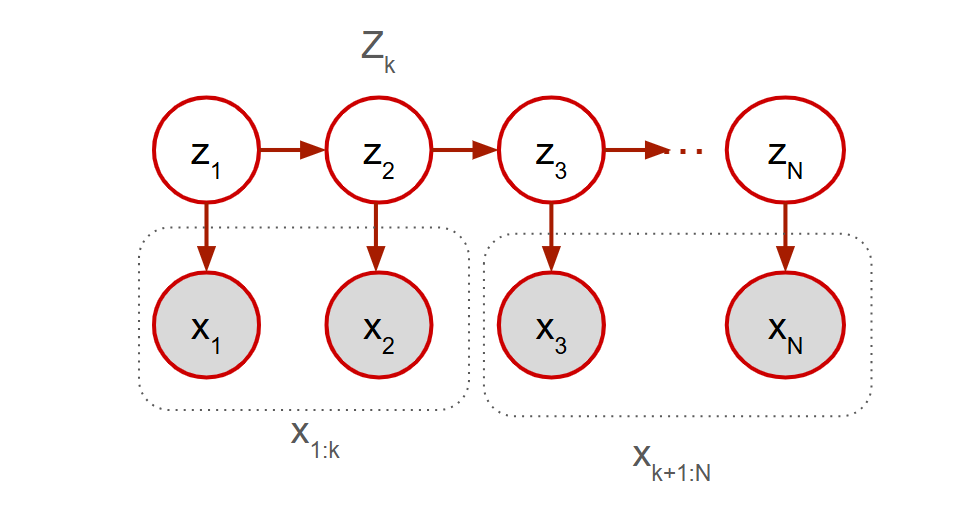
The observed variables are denoted by and the latent variables are denoted by .
- The joint PDF is given by .
- The values for are called emission probabilities governed by where is a probability distribution on (a PDF or a PMF).
- Notice the JPDF of the latent variables . The values for are called transition probabilities governed by a transition matrix where . Additionally, is called the probability of the initial state
Section 2.3: The Forward Backward algorithm
A key part in working with HMMs is the forward-backward algorithm that uses dynamic programming. Assume that the are known, we want to compute . We know that the joint PDF is given by 1 above
\\
Given , is independent of since it is d-separated by
Backward Forward
Using this extimate for , we can either (a) estimate “inference” probabilities, (b) Sample from the posterior (c) In the Baum-Welsch algorithm for estimating the HMM parameters.
Forward algorithm
The forward algorithm is used to compute . To do this we try to incorporate both to bring in the transition probabilities and to bring in the emission probabilities.
\\ Inc. and marg over that has M possible states
\\ splitting
\\ P(A, B) = P(A|B)P(B)
\\ P(A, B) = P(A|B)P(B)
for
Without DP, the cost of computing all = M (for each possible state of ) x M (summation in the equation for ) x N (number of observations)
Backward algorithm
\\ Chain rule : P(A, B, C, D) = P(A | B, C, D) P(B | C, D) P(C | D) P(D)
for
Section 2.4: The Viterbi algorithm
The Viterbi algorithm is used to determine the most likely (path of) hidden variable states given the entire sequence of observations. Let’s call (Note that ) the most likely sequence of z’s given all the observations .
To compute , we need to estimate
To break this down recursively (to use dynamic programming), we define a
\\ P(A, B) = P(A|B)P(B)
\\ Chain rule : P(A, B | C) = P(A | B, C) P(B | C), terms cancelled due to markov assumption
Where
Finally, to link back,
More on applications and practical guides in another post!
[1] Bishop - Pattern Recognition And Machine Learning
[2] 🔗 YouTube - Pattern Recognition & Machine Learning